by Michael Cropper | Jan 15, 2015 | Data and Analytics, Digital Marketing, Events, PPC, SEO, Social Media, Technical, Tracking |
Just before Xmas I was invited to speak at the Creative Entrepreneur event at Media City in Manchester to share insights into how online retail is changing. In-between speaking, it was great to listen to other online retail experts to hear their thoughts about where things are heading. So we can take a look through some of the discussions points in this blog post.

ASDA
First up we heard from Dom Burch, the serial speaker and senior director or marketing innovation and new revenue at Walmart UK (Asda). He shared his insights into how some of ASDA’s recent campaigns have been hugely successful in many aspects online and offline.
Dom’s first tip was around innovation and the importance of innovating throughout your entire business, regardless of how big or small you are. Innovation is key to long term and sustained growth. Simply dipping a toe in the water isn’t going to cut it here, Dom advised that you need to be giving projects at least 6 months to succeed (or fail!) so that you can be confident that you have exhausted all possibilities for the idea and had the time to gather data and assess the results accurately.
With all innovative ideas, you are starting with a goal of some kind for the business. Starting with ambitions to “become a big business” is equivalent to starting with the idea of “making a video go viral”. It’s simply the wrong approach to take and will inevitably lead to disappointment as goals are not hit. Instead, start with goals that are relevant for your business, goals that are in-line with your customer demands and goals that you can actually influence.
In between these ideas, Dom shared a few interesting statistics about ASDA;
- ASDA FM listeners have more people listening that Radio 1 and Radio 2 combined
- There are over 18 million customers who visit ASDA stores weekly
- ASDA’s website has over 300 million impressions every month
These are quite similar figures to what was announced last year at a digital marketing conference in Manchester.
With ASDA spending over £100 million per annum on broadcasting adverts, Dom’s approach was to get the PR team using Twitter, which was quite a challenge. Spending as little as 2 hours per week on Twitter, the newbie-to-Twitter PR team were already having a conversation with the editor of Vogue within 2 weeks. Where else could you get this kind of conversation going in 2 weeks? It simply wouldn’t be possible.
Another tip came in the form of doing something yourself first so that you know how to do it. This is something that I firmly believe in personally and in business. If you don’t at least understand what is happening, how can you ever hope to really manage this process? This is not to say you need to be an expert in every aspect as this would be impossible. Instead, it is hugely important to get a good grasp on every aspect within business and digital so that you can fully understand why things are being implemented and the reach they will ultimately have.
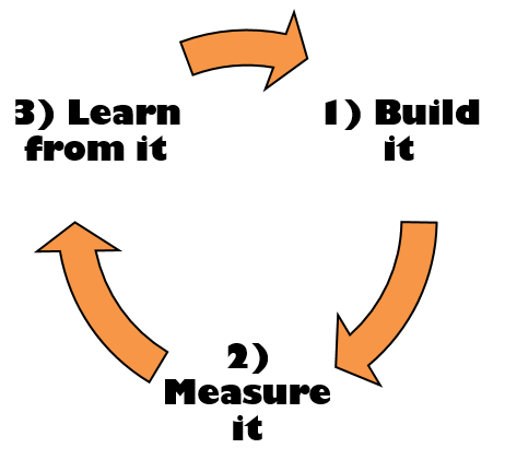
The simple process above will help you to build fast, fail quickly and innovate throughout your business at speeds you have never done before. Ideas are worthless, implementation is key and the only way to see what does and doesn’t work is to loop through the process as fast as possible, while giving every idea the time and energy to succeed.
Have a think for a moment, what are the 10 ideas that you have been talking about in your business last year? I can guarantee that there will certainly have been more than 10 ideas, but what were the 10 most important ideas? How many of these have you actually implemented, 5, 3, 1, none? Start the year off as you mean to go on. Run through these 10 ideas and measure everything to see how they impact your business. Capture the data and make informed decisions about the success of each campaign or idea.
For established businesses like ASDA, they aim to spend between 1-5% of their marketing budget on what Dom called “Trial and Error” campaigns which may or may not work. For businesses within the SME market, I would suggest this should be much higher as you are often still in the stages of experimenting with campaigns to see what works for your business. We naturally review and manage a lot of campaigns in the day to day work we do, although even we cannot tell you with 100% accuracy what will or won’t work for your individual business. We can certainly take into account the years of expertise and make a highly educated decision, although every business and every customer is different.
ASDA know that 74% of their customers are on Facebook, 20% are on Twitter and 15% of their customers watch YouTube daily. This information allows ASDA to invest their digital marketing spend in the right areas and not simply spend money on ‘more followers’ with no engagements. Their YouTube strategy focuses on how-to style videos and researching products which are broken down into 3 main groups;
- Hygiene content: Something that is core to what you do and for your core target market
- Hub content: Regularly created content designed to push this in front of your audience
- Hero content: Large scale campaigns to raise brand awareness, think about the epic Volvo Trucks campaign
The next of ASDA’s campaigns that was shared was with the involvement of Tanya Burr. Who you ask? Ask your teenage daughter if you have one. If you don’t, like me, then I also had to Google her to find out a bit more about her! She is described as a “Beauty, Fashion, Baking, Lifestyle Blogger & YouTuber” in a nutshell. And more than that, she has 1.2 million followers on Twitter. This is the reason ASDA worked with her, to reach this huge audience. The reach that ASDA’s products gained on social media was astronomical, just take a look through the number of views for each video that they produced together and you will start to understand how collaborations like this can pay off. Where else could you gain that kind of reach? To put things into context, Game of Thrones receives around 1.3 million views every week, which is less than what ASDA managed to reach with this collaboration. Likewise, Tanya Burr has more followers on Twitter than Sheryl Cole, Madonna and BBC Radio 1. Just because you have likely never heard of people like Tanya, doesn’t mean that they aren’t hugely successful.
When looking at YouTube videos specifically, always keep an eye out on the engagement levels and not simply the number of views of a video. Any brands that have a lot of views yet very few likes/dislikes means that they have likely paid a lot of money to drive traffic to the YouTube video and no-one liked it so they just bounced straight back out again. High engagement levels allow you to listen directly to your customers in ways like never before. ASDA’s videos with Tanya weren’t simply ‘buy this product’ videos, that’s boring and a fast way to drive customers away. Instead, they focused on food, health and wellness, beauty and style.
ASDA took this whole campaign one step further by creating the Mums Eye View YouTube channel which linked together their partnerships with Tanya Burr, Zoella and the Lean Machines. Google them all to grasp the scale of what is being achieved with strategic partnerships. This is a very young audience that ASDA was targeting here and one that has clearly paid off. With reports of as little as 2p per view of a YouTube video, 70% retention rate, 4 minutes minimum viewing time with an average of 7 minutes in length per video. You could only achieve these results with effective digital marketing that focuses directly on your customers. Not once did ASDA think “let’s make this video go viral”. What this also shows is that people like long form content on the web. No more do videos have to be 2 minutes in length, don’t be afraid of pushing the boundaries to meet customer demands.
This brings us nicely onto newspapers and traditional newspaper advertising. Quite frankly, no-one reads newspapers anymore, and I don’t say that lightly. Ask yourself, when was the last time you bought a newspaper? Personally, I can’t remember the last time I bought one, other than on the occasional times when I’m featured in one to keep as a little memento. Keep everything into context, could you seriously generate a response of someone looking at your advert for 4 minutes in a newspaper? I don’t need to answer that for you, it is clear. For ASDA, they know that 4/5 people don’t shop in ASDA and that is OK. So why spend £150,000 on a single press release in a national newspaper when 4/5 people of the people still reading newspapers aren’t ever going to be interested in ASDA anyway?
The summary of Dom’s keynote speech was that brands and businesses need to take a step back and see what is happening in the world. It’s time to start creating more content that relates to your audience.
Cyber Security
The next session was all about cyber security and the steps you can take to protect yourself. You need to look no further than the recent headlines about how many companies have been hacked into last year with millions of customer details stolen; eBay, Sony, Moonpig and endless more including 273 million customer details stolen from Yahoo and 250,000 customer details stolen from Twitter.
Some interesting statistics announced around cybercrime included that it costs the UK economy over £6.8 billion per year and the global economy £238 billion annually. With 81% of large businesses having experienced security breaches in 2014. The cost of a typical breach is now at £1.15 million, up from £600,000 in the previous year.
Some of the most common attacks are due to very basic hacking just after Update Tuesday. Windows PCs are updated every Tuesday with security patches that have been identified to keep your system and data safe and secure, yet so many people either ignore the messages on their computers or simply turn off the automatic updates. This is mad! As part of the weekly update from Microsoft, the hackers use this information as a shopping list of exploits on computers around the world they can attempt to get access to. If your system isn’t up to date, then you could be at risk.
Moving onto more sophisticated attacks such as DDoS attacks, which stands for Distributed Denial of Service attacks, these can bring down websites with ease. To the point at which you can actually purchase an attack on the black market to target a specific website for a specific amount of time. Unlawful and illegal hacking is turning into an underground commercial business. DDoS attacks are actually quite simple;

This method for DDoS are often using thousands, hundreds of thousands if not millions of computers from around the globe. For example, here you can see a short visualisation of a DDoS attack happening in real time on my personal blog a couple of years ago;
Have a read more about the full details if you are interested. The exact same thing happened to Mastercard, Visa and PayPal when they decided to stop sending funds through to the hacker group Anonymous. Whether you agree or disagree with this is another discussion all together and one that doesn’t have a simple answer. The important point here is that DDoS attacks are a real and present threat for businesses. While it is unlikely that you will encounter the wrath of some of the more prolific public hacking groups, the reality is that a lot of business websites for SMEs are hosted on cheap and nasty web servers that are poorly configured and have very little security built into them. Make sure your web server has the right protection in place to at least minimise the chances of DDoS attacks affecting you. The unfortunate reality is that if someone is determined enough to bring your website down, they will do. You can make it harder for this to happen though by having the right infrastructure in place for your website. Aren’t sure if your website and web server is protected? Then get in touch and we can review to check for vulnerabilities.
Moving away from hacking and looking at other types of data breaches now. Some of the most common data breaches often come in much simpler formats and often due to human error, aka. lack of awareness about threats. Threats including basic passwords on mobile and tablet devices to avoid automatic access to cloud based file storage systems for your company if a device is lot of stolen, to a deeper understanding of programming languages to avoid rookie mistakes.
Website vulnerabilities in particular happen for a number of reasons including unpatched software/content management systems/plugins, poor coding practices, poor server configuration, unencrypted data and more. Getting all of the above right is the absolute minimum businesses should be doing. Simply having a website built and not thinking about on-going updates is madness with how easy it is to exploit unloved websites. Every website should have regular and on-going maintenance to keep the website, content and data secure.
As of this year, there will be new EU Data Protection legislation that will be coming into force that businesses must adhere to. All of which is designed to move the current legislation into the digital age where customer data is collected at an alarming rate, often with very little visibility about what is being collected. This is likely to include full disclosure when data breaches happen so that customers are aware of what has happened. Far too often, businesses try and sweep large data breaches under the rug and hope that no-one will notice.
During the session, a live demonstration was given showing how easy it is for someone to steal your details – Even with my background, I was surprised at the level of things that can be done to steal personal details without you ever knowing what has happened. For example, simple things like clicking a link in an email can allow hackers to steal all of your saved login information in your browser. It really is that simple. Likewise, downloading a seemingly normal looking file from an untrusted source can result in a Key Logger being installed on your computer which will then be able to ‘read’ every single key you press, including your online bank account details and email passwords.
You may have heard about the infamous Stuxnet virus that swept the world almost by stealth last year. If you haven’t, you really need to read a few articles about this serious security threat; Wired, Business Insider, Wikipedia and what is even more worrying is that the source code for the virus is now publicly available on certain websites. As a quick overview if you haven’t come across Stuxnet before, the virus was designed specifically to find a physical controller located in power plants that controlled the heating/cooling of the nuclear material. As you can imagine, hacking into this and reporting an incorrect figure would lead to catastrophic results. This shows how sophisticated hacking has become. Some sources say that the virus was created by the US to target Iran’s nuclear facilities – how true this is, I don’t know. Other notable viruses including Duqu and Flame again highlight the level of sophistication that is happening right now.
Other common hacking attacks include the likes of SQL Injection attacks and Cross Site Scripting (XSS) attacks. Have a read up on these, again hugely important issues to be aware of and protect yourself against. Inexperienced and junior people working in digital are often oblivious to all of this type of information and most importantly how to protect against it. Always work with a company and people who are professional and have a very deep understanding of the industry they are working on. Remember the quote “If you think it’s expensive to hire a professional to do the job, wait until you hire an amateur”.
Now can you see why it is important to keep your systems, website and servers secure? Good, I’m glad the message has been received. If you don’t know what to do next, then get in touch and let’s have a chat.
Online Retail Panel

Next up was the panel that I was part of alongside three other digital agency owners in Manchester and London along with the Head of Online Retail for Iceland Foods, Andy Thompson. The session took a rather interesting turn to talk around a lot of digital topics about business growth through online retail, internal communication challenges and solutions along with some blindingly obvious opportunities for large brands to improve their sales online. The talks should be going online once they have been edited which you can look forward to watching, so for the meantime, here is a quick summary of the whole event and more information can also be found on the website;

Digital Marketing, SEO and the Internet of Things
The last few sessions of the day are combined within this section. We heard from many different speakers and panellists in the final sessions with lots of great tips for businesses. One key message that is extremely relevant for the SME market is that you simply can’t have social media accounts without creative content. You need to be creating your own content and sharing this socially along with utilising other great content around the web to fuel your social media channels.
The Tales of Things by Oxfam
Oxfam was involved in a very interesting project with the University of Salford titled The Tales of Things. Oxfam have invested £1.4 million over the past 3 years with the aim of revolutionising business systems and processes through the use of digital technologies. The Tales of Things project was a very interesting one and one which I believe we will start to see more of over the next few years.
The idea was around selling donated products that also have a QR code attached to them. Customers looking at the item would then scan the QR code to listen to a short story from the person who donated the item. Oxfam found that this actually increased sales by 57% in the Manchester shop. They then extended this into Selfridges in London where celebrities donated items with the same concept behind. Within 14 weeks, they had this technology applied in 10 Manchester shops. This is ultimately a historical archive for objects that are traded, thus turning an object into something more than an object as it has a story behind it.
Personally I hate QR codes with a passion due to the way that they are misused in 99% of circumstances by businesses. Although in this instance with Oxfam, this is a really great way to bring things to live and genuinely adds value to the product being purchased and the customer experience.
This project has been on-going for a few years now so have a good read about the finer details over at the BBC, Oxfam and Tales of Things.
Cool Tech
Where would we be without a blog post talking about some cool technology that is on the horizon? Here is a really cool digital air hockey game that Tom Cheesewright and I played (which I think I won, Tom may disagree, not that I’m competitive in any way! );
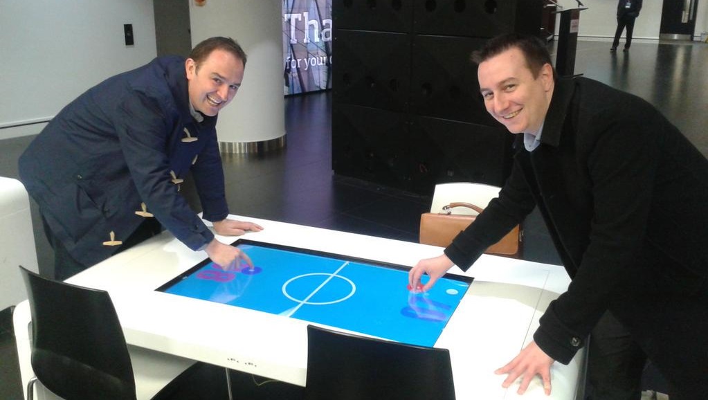
Image courtesy of Aleksej Heinze
And this was even more amazing, a 3D holographic projection (apologies for the poor quality, it was taken on my smartphone);
Summary of Event
Overall, the event was excellent with lots of great tips and advice to take away and implement. I’m sure there are a lot of questions about what you need to be focusing on in your business after the security discussions and digital marketing opportunities discussed above. Get in touch and we can talk things through with you to see how we can support the growth of your business.
Keep an eye out for next year’s event
by Michael Cropper | Jul 28, 2014 | Data and Analytics, Digital Marketing, News, Technical, Tracking |

That’s right, we’re now a Purple WiFi Authorised Reseller! You may be wondering just exactly what Purple WiFi is and why we have chosen to work with Purple WiFi. Before we go into that, let’s just look into the near future to see where the world is heading.
At some point in the near future, all business will start with some form of digital interaction. Whether this is business to business or business to consumer, or what is starting to be referred to as person to person. With smart technologies creeping into our daily lives from Google Glass, the Oculus Rift and a 3D printed mini me, we are seeing traditional online and offline areas blending into one. No longer is ‘digital’ a marketing channel that is completely separate to core business. For many businesses, ‘digital’ is becoming core business as brands start to interact with customers at every step along the way, from visiting physical stores to purchasing products on the website to connecting with customers on social media. Everything is digital.
For this reason, we predict that in the very near future, brands are simply going to have to join the dots for customers between all touch points, regardless of whether this is online or in the real world. That is why we have become a Purple WiFi Authorised Reseller, because the software is capable of joining these dots together which we believe are becoming increasingly important. Joining the online and offline worlds together in a way that has traditionally been extremely difficult for brands to do is now possible.
What is Purple WiFi?
Purple WiFi is extremely advanced and cutting edge technology that is designed to turn the current free WiFi in your premises into a marketing tool to directly increase revenue. To keep this really simple, Purple WiFi is a piece of software that is installed on your router (the ‘thing’ that connects your customers to the internet).

It is this software that gives your free WiFi the boost that is needed to which customers are in your premises, how many times they have visited before and how long they have stayed. In addition, you can see full customer demographic data including name, age, gender, email address and hometown. All of this amazing data allows you to understand who your customers are better than ever and communicate with them to increase the frequency of their visits. Get in touch with us to see a full list of the amazing demographic data you can capture with the tool or to request a demo.
Essentially, if a customer visits your venue once per month and we can turn this into them visiting once every two weeks through targeted email marketing, then this has doubled your revenue per head for that specific customer. It isn’t always about getting ‘new’ customers through the door, if you can achieve the same revenue growth from your current customers then this is also a good opportunity.
Why we have chosen to work with Purple WiFi?
Quite simply, Purple WiFi are the leading players in the market providing this software who are working extensively with global hardware manufacturers including Cisco, Linksys, NetGear, TP-Link, Cisco Meraki, Deliberant, HP, Mikrotik, Open-Mesh, Ruckus, Xirrus, Airtight Networks, Buffalo, Trendnet and Ubiquiti.
The Purple WiFi software works on the leading hardware solutions for your wireless network, meaning that you can be confident that you can start to benefit from this software sooner rather than later.
Turning Purple WiFi into our WiFi Marketing and Analytics Service
Purple WiFi on its own is great, but as with anything, if you don’t use the tool to its full advantage then you won’t get the most out of it. After speaking with a lot of businesses ranging from bars and restaurants to bowling alleys and shopping centres, one of the common themes coming from discussions is around the time it will take to manage the platform.
This is why we have created a service around Purple WiFi which we call ‘WiFi Marketing and Analytics’. It is this service that is designed for us to do look after the marketing part so you can focus on doing your job within the business. Instead of having to learn how to use another tool to maximise its potential, we will do that for you and use our expertise and knowledge of running multiple campaigns to get the best results for your business.
Whether you are simply looking to offer your own branded free WiFi solution for your customers, or whether you are looking to utilise this for a data capture tool, or even if you are looking for the full works to utilise all of the above and turn your free WiFi into a marketing tool to increase revenue. Whatever you are looking for, our WiFi Marketing and Analytics service can be tailored to your specific needs and we can talk you through how this works in practice within your own organisation.
Find out more about our WiFi Marketing and Analytics service over on our services page which talks you through how this works in more detail along with giving some ideal examples of how this new technology can be used to the full advantage. Purple WiFi only sell the software through authorised distributors like ourselves, so get in touch to find out how this can work for your business.
We don’t simply build websites. We work with your business to increase revenue through digital technologies, which just happens to include things like web design, search engine optimisation, pay per click advertising and now WiFi Marketing & Analytics. Get in touch if you would like to know more about how we can support the growth of your business through digital marketing and new technologies.
by Michael Cropper | Jun 7, 2014 | Developer, Technical |
Within our daily work we use Excel an awful lot, so naturally we like to use Excel to its full potential using lots of exciting formulas. One of the major challenges within Excel is trying to use a VLOOKUP function within a VLOOKUP function. In summary, this isn’t possible. The reason this isn’t possible is due to the way the VLOOKUP function works. Let’s remind ourselves what the VLOOKUP function actually does;
=VLOOKUP(lookup_value,table_array,col_index_num,range_lookup)
What this means in basic terms is “find me a specific cell within a table of data where a certain criteria is met”. This is such a powerful function that can be used to speed up work in so many different ways. But we aren’t going to look at why this is so great here, we are going to look at the main limitation and most importantly how to get around this with more clever magical Excel formulas.
Solutions
The solution to this is quite a complex one and one that involves many different Excel formulas including;
- =ROW()
- =INDEX()
- =SUMPRODUCT()
- =MAX()
- =ADDRESS()
- =SUBSTITUTE()
- =MATCH()
- =CONCATENATE()
Throughout this blog post we’ll look at what each of these mean and how they can all be used in conjunction to perform a function what is essentially equivalent to a VLOOKUP within a VLOOKUP.
The Data
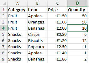
Before we jump into how to solve the problem of performing a VLOOKUP within a VLOOKUP, here is the data that we will be working with. Let’s assume that we have a large list of products which are associated with multiple different categories as can be seen below;
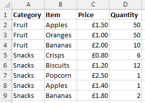
Data Sheet – Prices
You may be wondering why apples and bananas are classed as snacks in the data. Don’t worry about that. Just go with it. There are many different situations whereby you may be presented with this type of data so this is purely to illustrate the example in a simple way.
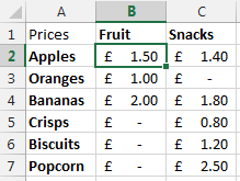
Now let’s say that you want to visualise this information a little easier. The above table of only 8 entries is reasonably straight forward. Although one example we’ve been recently working with had over 35,000 rows of data which was a little more challenging to view in this format and we wanted a simpler way of looking at this information within Excel. So let’s say we want to look at the data in the following way;
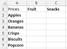
Data Sheet – Summary Prices
This is the data that we will be working with so you can clearly see how this technique can be implemented. To keep things easier to understand, these two pieces of data are kept on two separate sheets within the Excel worksheet.
Quick Answer
Looking for the quick answer to this complex formula? Then here is the answer;
=IFERROR(VLOOKUP($A2, INDIRECT(CONCATENATE(“‘Prices’!”, SUBSTITUTE(ADDRESS(MATCH(B$1, Prices!$A$1:$A$100, 0), 1), “A”, “B”), “:”, SUBSTITUTE(ADDRESS(ROW(INDEX(Prices!$A$2:$A$100,SUMPRODUCT(MAX((Prices!$A$2:$A$100=B$1)*ROW(Prices!$A$2:$A$100))-1))), 1), “A”, “D”))), 2, FALSE), 0)
You may be a little confused with the above, so this post will explain exactly what each part of this means and why it is contained within the rather large and complex formula above. Most importantly, you will be able to understand how to perform the equivalent of a VLOOKUP inside a VLOOKUP.
Steps
The individual steps within the above formula can be broken down into much smaller and easier to understand steps as can be seen below;
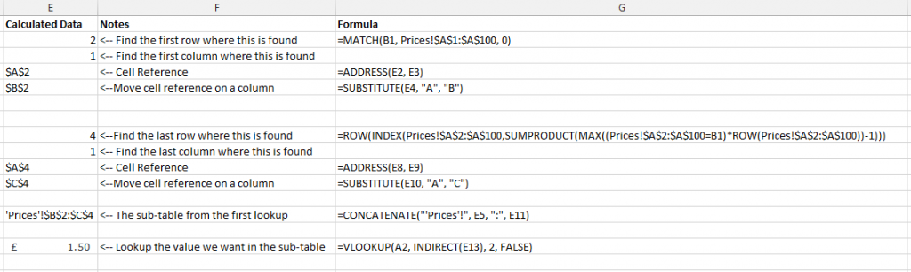
Steps for how to perform a VLOOKUP inside a VLOOKUP
Below we will talk through each of the above steps so you can understand why it is important.
Find the Sub-Table
Firstly if you are wanting to perform a VLOOKUP within a VLOOKUP then you need to find where the sub-table starts and ends. While you could manually enter this in for very small data sets, this is simply not practical for large data sets.
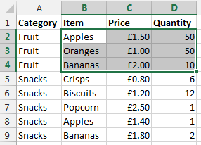
To perform this action we need to define search for the first and last occurrence of when ‘something’ is found. A note on this point, you will need to ensure that your lookup data, in this case the ‘Prices’ sheet, is ordered by the column you are looking up, in this case the ‘Category’ column. Since if this isn’t the case, then data will be included within this sub-table which shouldn’t be.
To do this, we need to find both the first occurrence and the last occurrence. What we are looking to achieve is identify the sub-table for ‘Fruit’ which can be seen below;
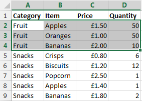
The sub-table we are looking for
Once this has been identified, then we can use the standard =VLOOKUP() function on this sub-table to find the data we would like.
Find the First Occurrence
There are a few different formulas included to find the first occurrence of data within a column which are outlined below.
=MATCH()
To find the first occurrence of ‘something’ within a range of data then we use the =MATCH() function. To remind ourselves of what the MATCH() function is, here is the official description from Microsoft;
The MATCH function searches for a specified item in a range of cells, and then returns the relative position of that item in the range. For example, if the range A1:A3 contains the values 5, 25, and 38, then the formula
=MATCH(25,A1:A3,0)
returns the number 2, because 25 is the second item in the range.
Use MATCH instead of one of the LOOKUP functions when you need the position of an item in a range instead of the item itself. For example, you might use the MATCH function to provide a value for the row_num argument of the INDEX function.
MATCH(lookup_value, lookup_array, [match_type])
Source
Looking back at our example, this translates into the formula;
=MATCH(B1, Prices!$A$1:$A$100, 0)
What this means is;
- Find the contents of B1, which is ‘Fruit’ in our example
- Within the range of data Prices!$A$1:$A$100
- And make sure it matches exactly (0)
This has now found the first occurrence of this information within the column of data. Now we need to translate this into something that a VLOOKUP formula can use.
=ADDRESS()
The next bit we need to look at is turning the row & column numbers into an ‘Address’ which Excel can understand. To do this we simple create the formula;
=ADDRESS(E2, E3)
The =ADDRESS() function takes a Row Number and a Column Number and turns that into an Address. In this case, the row number is generated from the previous function, =MATCH() and the value of E3 in the example above is 1. We use 1 because for this we are only interested in starting on the first column of data. Once we know we are starting here we can always move the cells along accordingly.
In our example, this address at this point in the large formula is set to $A$2.
=SUBSTITUTE()
Now we know we have created an Address in the previous step which was within column 1, this is also the same as column A. This makes life easy for us as we know where this is. The next step is to nudge the sub-table over so the =VLOOKUP() function can easily lookup the data in the later step.
To do this, we simply nudge the starting Address over to the right by one column using the following formula;
=SUBSTITUTE(E4, “A”, “B”)
Where E4 is the cell which contains the Address from the previous step.
The cell that has been identified as part of this step is the first occurrence as can be seen below;
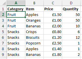
Find the first occurrence of data within the column
Now we want to nudge this over using the above function which will mean this item is now set to $B$2 which is the starting point of our sub-table.
Ok, so we now have the starting point for the sub-table for the VLOOKUP to use. We now need to calculate the end point so the sub-table can be used within the VLOOKUP.
Find the Last Occurrence
Finding the first occurrence of data in column is a lot easier than finding the last occurrence as you can see from the formula below that we need to do this;
=ROW(INDEX(Prices!$A$2:$A$100,SUMPRODUCT(MAX((Prices!$A$2:$A$100=B1)*ROW(Prices!$A$2:$A$100))-1)))
The key functions we need here are;
- =ROW() – Which takes a reference and calculates which row number this is on
- =INDEX() – Which returns a value or the reference to a value from within a table or range.
- =SUMPRODUCT() – This is used to tell Excel the calculations are an array and not an actual number
- =MAX() – This is used to find the largest row number in the array where the lookup value occurs
- =ROW() – This, as before, is pulling out the Row Number from the data retrieved
Unlike previously, it is not simple to break this out into sub-sections to explain the different points as the formulas don’t work when breaking them our separately due to the way the =SUMPRODUCT() function works. As such, I’ll talk through what each of the different parts of the formula mean and what they do.
=SUMPRODUCT(MAX((Prices!$A$2:$A$100=B1)*ROW(Prices!$A$2:$A$100))-1)
This formula is identifying the last occurrence of the data that is in cell B1 within the range of data $A$2:$A$100, which in our example is ‘Fruit’. We then wrap this in the =INDEX() function to get the cell reference then wrapping this in the =ROW() function which will identify the row number where this data is found;
=ROW(INDEX(Prices!$A$2:$A$100, SUMPRODUCT(MAX((Prices!$A$2:$A$100=B1)*ROW(Prices!$A$2:$A$100))-1)))
You may have spotted the -1 in the formula above. This is to ensure that the data is pulling back the correct row number. If this isn’t there, then you will notice that the data that is pulled back is a row below where you would expect.
To get a good understanding of the above part of the formula, then I’d recommend reading the fantastic guide over at Excel User.
What we have achieved using the above combination of formulas can be seen below as the last occurrence of data in the column;
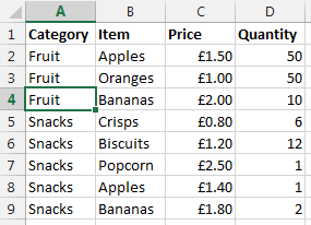
Find the last occurrence of data in the column
Once we have this data we then wrap this in an =ADDRESS() function then a =SUBSTITUTE() formula which first turns the result into an Address that Excel can understand, opposed to standard text, then moves the data over several columns from column A to column D. This is needed, since we will be creating a sub-table that includes several columns. In this case, 3 columns which are column B, C and D. If you are working with data with more columns, then you will need to replace the D with a higher column.
SUBSTITUTE(ADDRESS(ROW(INDEX(Prices!$A$2:$A$100,SUMPRODUCT(MAX((Prices!$A$2:$A$100=B$1)*ROW(Prices!$A$2:$A$100))-1))), 1), “A”, “D”)))
Move the column to the end so we can create a sub-table that contains all the required data
So now the end of the sub-table is set to $D$4 which means that we have a starting point and an end point for our sub-table which can be used in the =VLOOKUP() function as outlined below.
Lookup Data in the Sub-Table
Now we have the sub-table defined using all of the above formulas, we can use the standard =VLOOKUP() function once we have joined all of the above data together.
Create the lookup table
Now we have all of the above points, we need to create the lookup data using the standard =CONCATENATE() formula as can be seen below;
=CONCATENATE(“‘Prices’!”, E5, “:”, E11)
The data within E5 is the starting point of the sub-table, and the data within E11 is the end point within the sub-table. In our example, this gives us the answer of ‘Prices’!$B$2:$D$4.
Lookup data
Now we have the sub-table to lookup the data we want, we can simple use the standard =VLOOKUP() function to find the data that we require as follows;
=VLOOKUP(A2, INDIRECT(E13), 2, FALSE)
We wrap the concatenate function within the =INDIRECT() function so that the data is treated as a reference, opposed to text. The data within E13 is the result of all of the work previously in this post, I’ve just left this in here to make this easier to read and understand. For the full formula, this would be replaced with the individual parts. Now the data that is brought back is exactly what we want.
Sub-table of data based on initial criteria
What this final =VLOOKUP() function is doing is saying “find the value in A2 within the sub-table we have identified, then bring back the second column of data. So in our example, the long formula in column B1 is bringing back the data £1.50 as can be seen below;
Result of a VLOOKUP inside a VLOOKUP
Summary
So there you have it, how to perform the equivalent of a VLOOKUP within a VLOOKUP using a few different formulas within Excel. You may be a little scared of such a huge formula at first, but you will see that when you do need to use this, I would always recommend breaking this out into the different parts before trying to create one monolithic formula as you will be able to put this together much easier.
Also, in the formula below, you will notice that it is all wrapped in an =IFERROR() function which simply sets the data to 0 if nothing can be found. You can set this to whatever you like, I just chose 0 since this was about prices.
=IFERROR(VLOOKUP($A2, INDIRECT(CONCATENATE(“‘Prices’!”, SUBSTITUTE(ADDRESS(MATCH(B$1, Prices!$A$1:$A$100, 0), 1), “A”, “B”), “:”, SUBSTITUTE(ADDRESS(ROW(INDEX(Prices!$A$2:$A$100,SUMPRODUCT(MAX((Prices!$A$2:$A$100=B$1)*ROW(Prices!$A$2:$A$100))-1))), 1), “A”, “D”))), 2, FALSE), 0)
=IFERROR(VLOOKUP({Main-Lookup-Value}, INDIRECT(CONCATENATE(“‘{Sheet}‘!”, SUBSTITUTE(ADDRESS(MATCH({Sub-Table-Lookup-Value-First-Occurrence}, {Sheet}!{Sub-Table-Lookup-Range}, 0), 1), “A”, “B”), “:”, SUBSTITUTE(ADDRESS(ROW(INDEX({Sheet}!{Sub-Table-Lookup-Range},SUMPRODUCT(MAX(({Sheet}!{Sub-Table-Lookup-Range}={Sub-Table-Lookup-Value-Last-Occurrence})*ROW({Sheet}!{Sub-Table-Lookup-Range}))-1))), 1), “A”, “{Column-Letter-For-End-Of-Table}“))), 2, FALSE), 0)
Simple really!
Ok, so this isn’t for the faint hearted. But for those advanced Excel users around I’m sure you will have come across times when you really needed to perform a VLOOKUP inside a VLOOKUP and found that after a long time researching how to do this online that it isn’t a simple task. So hopefully you can see the clear steps included above and this will help in the future. The beauty of the above formula is that you can now drag this into new rows and new columns without having to update anything, all thanks to the $ signs throughout the formula.
by Michael Cropper | Sep 14, 2011 | Data and Analytics, SEO, Social Media, Technical, Tracking |

With the recent announcement from Bit.ly stating that their Pro version is now the normal version, this means that it is now possible to get your own custom short URL. But how though?
Step 1 – Register a nice short domain name
A good place to do this is 101Domain.com as you can get a nice view of all top level domains available, with the added bonus that they are very reasonably priced too. For mine I chose “mic.cx”. When looking on 101Domain.com you will notice they offer some great advice on the restrictions certain domains have, such as where the hosting or name servers have to be based so keep an eye on this when purchasing an odd top level domain.
Step 2 – Set up the DNS A record
When you log in to your registrar (the person you bought the domain from) there will be some settings somewhere that allow you to change the DNS records (not to be confused with the Name Servers). Here is an example of what this will look like

When you see this, change the IP address which is currently in there (may be worth making a note of this in case you mess up the first time like I did!) to the IP address “168.143.174.97” which is for Bit.ly. Other URL shortening services that offer this will have a different IP to enter, so check on their FAQ’s.
The “@” above, strangely, has no relation to email. It is referring to your domain in its purest form with no sub-domain. So for example that would mean mine is “http://mic.cx”
The “www” is referring to the URL “http://www.mic.cx” – but since Bit.ly doesn’t use this, then there is no real need to put this in – although I have done anyway for good luck.
Be aware that once you have updated the DNS settings this can take around 24-48 hrs to propagate the internet so be patient!
Step 3 – Add Custom Short Domain to Bit.ly
The next step is to go to Bit.ly (i’m assuming you already have an account at this point – if not sign up!) and click on the “settings” link from the drop down where your username is. Then add in your new URL into the box provided and go to the next step.

Step 4 – Verify Your New Domain

Step 5 – Success!
