Last week we attended the Future Cities symposium at Manchester School of Architecture which was talking about how the future smart cities are going to look and what is being done about this right now. Fascinating event and great to see how local councils are already starting to think through how technology is going to transform the world we live in. Over the next 5-10 years, I predict that the world we live in will be unrecognisable. The amount of development into smart cities, superfast internet and the internet of things is going to significantly change how the general public interact with the physical world around them.
The speakers at the event ranged from architects, directors of technology strategy boards and futurists. Below we will talk through the key topics that were brought up throughout the day and what this means for businesses and councils in the future.
Rory Hyde
Rory Hyde
The first speaker of the day was Rory Hyde, the curator of Contemporary Architecture and Urbanism at the V&A in London along with the author of the book Future Practice.
Rory opened the talks by saying that architects suffer from a “crisis of relevance” which he said wasn’t just about creating buildings but instead about being relevant for the space where the building lives and for the users of the building. He talked about 4 retreats from solid relevance including;
1) Avant-garde: Which is to try new and experimental ideas within architecture
2) Commerce: Currently developers often set the agenda, not the architects which often leads to extravagant developments that you can see throughout Dubai
3) Icons: Where architects often seek to chase new and exciting shapes of buildings to truly stand out from the crowd. Take for example the Burj Khalifa in Dubai, The Gherkin in London and Sydney Opera House
4) Urban interventions: Looking at personal utopias with clearly fenced off areas from the outside world
Looking into the future, Rory talked through ideas around schools and the availability of rooms and facilities. Imagine an ‘Airbnb for schools’, whereby everyone could get automatically updated with what is happening, information sent directly to their smartphones. If you haven’t heard of Airbnb yet, then it is the hotel booking website that is seriously disrupting the travel industry. The online service allows people to rent out their homes or spare bedrooms through the service. Launching only 6 years ago in 2008, they already have over 550,000 listings in 192 countries and will soon have more availability than the Hilton Worldwide and InterContinental Hotels Group globally. Imagine a system that knew when meeting rooms in a city were free and available for people, that knew when the buses were due so you could be directed to the most relevant place for you.
Smart Schools
An interesting point Rory made was around the idea of community architecture such as wind turbines. Often these are installed by large corporations which provide no benefit to the local communities. Which is often one of the reasons why there is so much negativity towards new installations. Instead, imagine a situations whereby local communities directly benefitted from new installations which provided revenue to support local services. This would significantly change the perception of these technologies and would benefit local communities far more.
Following on from this, talk was around a future city that blended with nature. The example given was from Studio Gang’s Bubbly Creek which would allow nature and city to merge together into a natural symbiotic system;
While this is an interesting concept, personally I’m not too sure this would work to the extent described in the plans. What is interesting though how future cities are significantly changing as traditional industries are often dwindling in size and scale. Less space is taken up as production increases which is leading to a hollowing out of the traditional urban core.
Tom Cheesewright
Tom Cheesewright
The next speaker of the day was Tom Cheesewright talking about how the future smart city will blend seamlessly with digital technologies. Tom is an Applied Futurist at Book of the Future.
Tom started his talk off by asking the question that if the current technology is affordable and accessible, along with data being cheap then why are smart cities and home automation such a challenge to crack? It comes down to user experience, he stated that “user experience is the last hurdle to for truly smarter cities”.
Smart cities today are essentially technology applied to the build environment to reduce the expenditure and increase efficiencies. This isn’t difficult, it just requires a significantly different approach to thinking about how the systems within the city are used and accessed by the users.
To prove the point, Tom has started to turn his house into a Smart Home with the use of cheap technologies such as the Arduino and Raspberry Pi. Basic implementation initially with automatically turning the lights on and off when entering or leaving a room. The point being that this technology is available now. The future smart city is possible now, when this technology is used throughout.
Arduino and Raspberry Pi
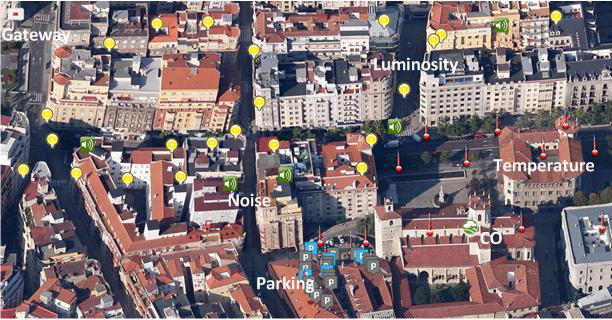
Taking this to a whole new level, the Santander Smart City in Spain. The project in Santander is a world first city-scale experimental research system for future smart cities. The project is designed to stimulate the development of future applications for users within the city. As part of the project, over 20,000 sensors were fitted across the city to monitor data across a wide range of points.
To give you an idea of the scale of this setup, here are a few statistics;
Around 3000 IEEE 802.15.4 devices
200 GPRS modules
2000 joint RFID tag / QR code labels deployed on streetlights, bus-stops, busses and taxis
Environmental monitoring with around 2000 Internet of Things devices installed to monitor temperature, noise, lighting and car presence
Outdoor parking area management with almost 400 parking sensors used to identify empty and full car parking spaces throughout the city
Sensors installed in over 150 public vehicles including busses, taxis and police cars
Traffic intensity monitoring with around 60 devices located at the main entrances of the city which are designed to monitor traffic volumes, road occupancy, vehicle speed and queue length
Guidance to free parking spaces which link up the live data from the 400 parking sensors with 10 street panels showing exactly which parking lots have spaces
Parks and gardens irrigation with around 50 devices being deployed in city green zones to monitor moisture temperature, humidity, pluviometer (aka. a rain gauge) and anemometer (aka. a wind speed monitoring device)
And much, much more, read the full details over on their website
Santander Spain Smart City
I’m sure you will agree that this is seriously cool. Exciting times ahead with future cities on the horizon. This isn’t a simple and quick fix for cities and towns to implement, although this is going to happen in the near future. The reason why this is the direction we are heading in comes down to resource planning, reducing costs and waste while improving efficiencies. Some of the statistics that Tom mentioned through his talk included how sensors placed in bins reduced the fuel bills for the council by 25% by simply only emptying the bins that needed emptying along with how the parking sensors and signs saved approximately 8 minutes for how long it took people to find a car parking space in the city.
Smart cities of the future will be context aware systems that optimise the build environment for its inhabitants. No longer will people have to go elsewhere to find out information about where they already are. This is interesting as we should start to be prepared for a post screen environment which allows people to interact with the city without being tied to a specific device with a screen.
Smart Cities Data and Processes
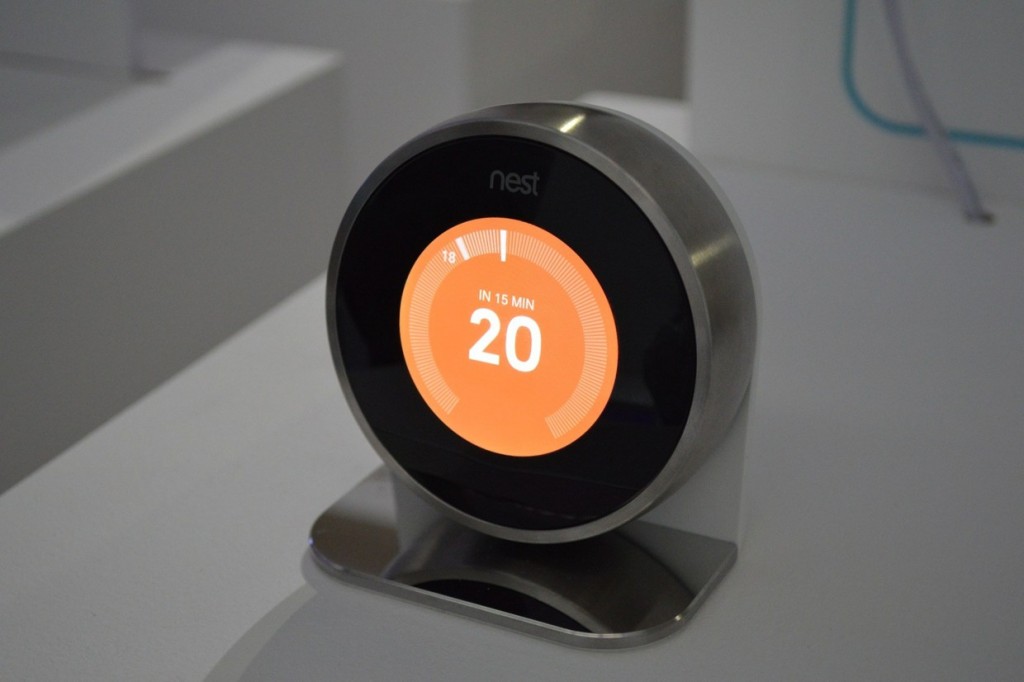
Whenever anyone talks about smart cities and home automation, we always have to mention Nest, Google’s recent acquisition. This is really important though as Nest claim that their US customers save on average 20% on their energy bills. This isn’t just about cool tech, well ok, it is partially, but it is also about how this new technology can have a significant improvement on current technologies to save money for people and businesses.
Nest Thermostat
The smart cities go beyond a reactive system. Imagine local councils knowing the actual noise and traffic levels produced from a factory near to a housing estate. Understanding this system allows the council to start to plan the towns and cities intelligently by using this environment and social feedback from the smart city technologies.
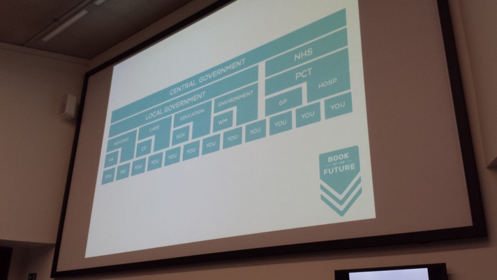
Tom went on to talk about the idea of connected councils where public services are reoriented around the citizen by connecting disparate data system to present a consistent and context aware experience for users. This is what Tom labels as “citizen centric design” which is all about the user opposed to a service centric design.
The main driving force for councils is to increase efficiencies, increase capabilities, increase satisfaction and increase engagement from the citizens. Smart cities work towards all of these goals. One example given, albeit a rather 1984 approach, was for adult care services. For example, if there are two call outs for environmental services at a property, there is a likelihood that adult care services should visit to see if there is any help needed.
Currently these conversations will be happening already in the council although more of a manual process whereby person A will walk over to person B in another department and mention it over making a coffee in the morning. The ability with smarter systems means that people don’t have to be used for the process, the system is used for the process. Meaning that people can be used for productive and value added work such as actually talking to the end users in this example.
Citizen centric design is designed to integrate data platforms and publish public APIs, allow for smarter strategic procurement which looks at the system as a whole, not just a specific job or department which will always lead to disparate systems being created. Using a hybrid agile development process for digital engagement skills and processes. Most importantly user testing, not simply pushing new technologies onto citizens
Current service centric design approach
Citizen centric design
Dan Hill
Dan Hill
Next up we heard from Dan Hill, the Executive Director of Futures and Best Practice at the Technology Strategy Boards Future Cities Catapult. Dan started his talk by stating that we need to understand that a city isn’t a static environment where changes can be made periodically, instead the city is a real time system that we need to tap into.
Dan gave the example of Masdar smart city in Dubai which is best explained through this concept video from a few years ago;
Really interesting how leading cities are grasping the idea of smart cities and capitalising on this opportunity. While this is still under development, this is certainly an interesting way smart cities are taking shape.
One interesting point that Dan expanded on was that we don’t make cities in order to build infrastructure. Often cities are designed with an infrastructure led approach. Instead, he argued, that we build cities for culture, commerce, community, conviviality and the city itself.
When designing on an infrastructure led approach, the design lifetime of an infrastructure is often planned out to be 100 years such as for a metro system, which in reality is often much less when change of government comes into play. With digital you are lucky if a website stands the test of time of 100 weeks before it is out of date. This means that digital systems have to be able to adapt at a much faster rate than ever before.
Dan went on to talk about the value and cost of inefficient systems that smart cities could improve upon. Quoting Cedric Price with “Technology is the answer, but what is the question?” The question was raised that if we have made it clear to citizens the value of a smart city to them. I would argue that we haven’t which is why privacy concerns are often at the forefront of people’s minds.
An interesting The Museum of the Future in the UAE showcases how cities will look in the future;
Museum of the Future
Really interesting concept looking at future cities and future technologies and how this will significantly change the world we live in and aid citizens with their daily life.
An interesting term was around “Urban Prototyping” which is all around creating products and services for the 21st century city and urban space. Looking at what citizens need within a modern city and looking at creating products and services specifically for these people.
Another project talked about was Sensing London which follows a similar theme around creating a smarter data driven city. The project is designed with three points in mind;
Collecting data for insight
Mashing data for innovation
Trailing innovations in real city environments
With something much closer to home, it will be interesting to watch how this project progresses over the next few years. Another piece of technology mentioned was DisplayAnts which is designed to create interactive public displays with public information available.
Dan then went on to talk about how software and hardware is blending with the use of smart software to unlock vacant resources in the city. With one recent example being the Uber taxi app that has been spreading around the world. Interestingly too is that this new technology isn’t always welcomed with open arms with Uber getting a lot of criticism in both London and Spain from angry taxi drivers, bringing the locations to a standstill. If you aren’t familiar with Uber, it is the taxi booking app that connects you as a customer with a taxi with the click of a button and is really disrupting the traditional idea of booking a taxi. This type of disruptive technology is going to continue to increase over the coming years in a range of industries.
Another interesting piece of information was about research from MIT which stated that we could have 80% fewer vehicles on our roads if we were using smart cars. This is an enormous saving and one that I’m sure any commuter would appreciate. Then going beyond smart cities, Bridj was mentioned which is not just looking at real time data, but predictive data based on historic information and demands. Essentially allowing more resources to be deployed in an area that is likely to need more resources soon.
Beyond this, we have the likes of KickStarter for more product based ideas. Well we also have BrickStarter which takes the same concept but looks at projects for cities and the urban environment. Interesting idea for allowing citizens to essentially pitch ideas in their local communities.
All this being said, we still have a long way to come, with planning notices still being tied to lampposts. This is still seen as the best way to engage with the public about work that is happening in an area. Quite frankly, this is a joke. 99% of people simply walk past this and take no notice at all. This is not a good way to be engaging with citizens within a local area.
Planning Notice on Lamppost
Final Thoughts
The smart city is coming. This also requires a new approach within governments and local councils to fully understand how this change is going to impact the world we live in. Education is also going to be key to ensure the citizens fully understand what the smart city is, why it is so valuable and most importantly teaching people about a new way of interacting with official bodies.
One final thought to leave you with, imagine in the near future with a publically accessible CityAPI, maybe powered by things such as Fi-Ware. Whereby you can easily plug your business into this system to send and receive data that is essential for you and your customers. We already have cool WiFi Marketing & Analytics technology available for businesses, so this is an even more exciting time ahead in a digitally enabled world.
With tools as powerful as Google Analytics at our fingertips, surely every business is measuring the results from their marketing activities? Well, in our experience, even large and well established companies find it difficult to track marketing activities accurately.
What this means is that marketing budgets are often not spent as effectively as they could be. This would be fine if all businesses had an unlimited marketing budget, but this isn’t the case. Marketing budgets are always limited, which means that businesses need to be investing in marketing channels that are performing well for their business.
Throughout this blog post we will talk through the different ways you can track your marketing activities effectively which will mean you can make smarter data driven business decisions. Tracking marketing activities accurately means you can invest further in activities that are working well for your business and stop spending money on activities that aren’t generating a return.
All of the items we are going to talk about within this blog post are possible to track with ease through Google Analytics.
Set up Goals
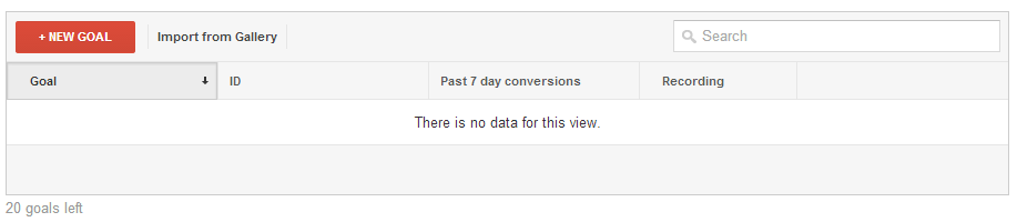
What is the main goal you want website visitors to do? It is to purchase a product, enquire about the services or solutions you provide, or do you want them to download a guide from your website? Within Google Analytics you can set up a maximum of 20 goals within Google Analytics, which means that you can track an awful lot of data;
Set up Goals within Google Analytics
To track your marketing activities accurately this is absolutely essential to set up useful goals for your website. This can vary hugely between different websites based on what you are trying to achieve. Although have a think about both macro and micro goals on your website. What are the key things you want your website visitors to do?
Contact us
Request a call back
Follow you on social media channels
Purchase a product
Download a resource or guide
Find a local branch or store
Click and collect
Once you fully understand what you would like your website visitors to do, then you can start to track your marketing activities accurately. Quite simply, if you are paying for website visitors that aren’t working towards your key goals then maybe it is worth spending the marketing budget in areas that are working towards those goals instead.
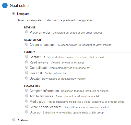
Within Google Analytics, setting up goals couldn’t be easier with the many templates that are already available for you to customise for your individual website;
Goal Templates within Google Analytics
Use Goal Funnels
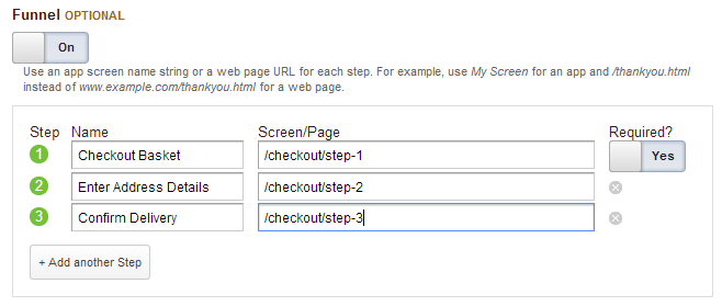
When you are setting up your goals above then you will be asked if you would like to use Goal Funnels. These are the specific steps that customers must go through before completing a goal. For example, if you are selling products online, then you will have multiple steps in the checkout process.
It is essential to set up the correct tracking for your purchasing funnel so you can understand how customers are behaving when they are completing this process. Below you can see an example for how this can be set up;
Goal Funnel Options within Google Analytics
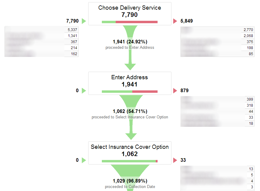
Once you have configured this correctly you can easily visualise this information within Google Analytics. This will show you exactly how your website visitors are behaving and most importantly, where they are dropping out of the purchasing funnel. This is invaluable data that can provide insights into where improvements can be made to increase the number of people who complete their purchases.
Funnel Visualisation in Google Analytics
This data shows you the number of people who move on to the next step in the purchasing funnel and it will also show you the number of people who leave the purchasing funnel. More importantly, it will tell you where they went. Did they go to another page on the website for further information, or did they leave the website completely? This information can really help to understand your customer behaviours and look for ways of improving the user experience.
Ecommerce Tracking
If you are selling any products or services through your website, then setting up ecommerce tracking within Google Analytics is absolutely essential. The data that this provides means that you can easily see which products and services are the most popular, and most importantly, which traffic sources are leading to customers purchasing.
Understanding which traffic sources are working best for your business means that you can then readjust your marketing budgets towards the most profitable areas. Only through correct tracking is this possible. Below you can see some of the useful data that you will start to receive once you implement ecommerce tracking on your website and in Google Analytics;
Ecommerce Tracking within Google Analytics
Just as with goal tracking, the important point here is that once you fully understand which traffic sources and marketing activities are working towards increasing sales through your website, then you can start doing more of this. All of which is essential to fully understand how your marketing activities are performing.
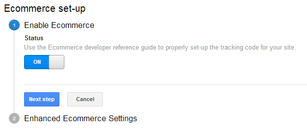
Implementing ecommerce tracking is a little more involved than setting up goal tracking. Firstly you have to enable ecommerce tracking within Google Analytics then also implement additional tracking codes on your checkout completion page;
Ecommerce Setup within Google Analytics
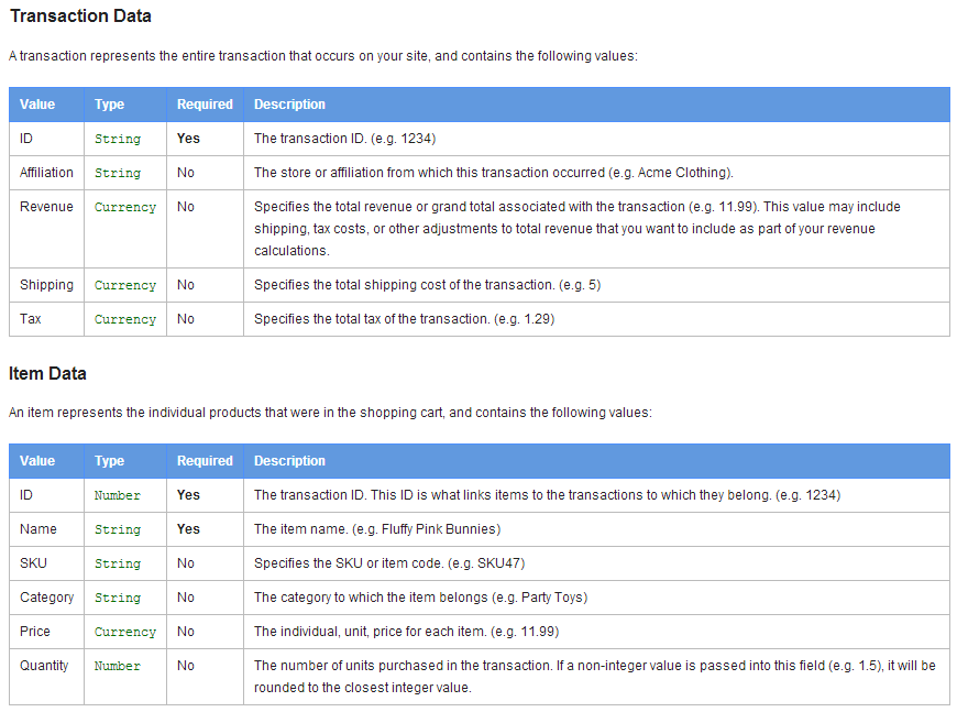
To learn more about how ecommerce tracking can be set up, it is recommended that your website developer reads through the following guidelines from Google. To summarise the requirements, there needs to be additional information on the checkout complete page that contains all of the following information so that Google Analytics can pick this up and fire the data into the reporting platform;
Ecommerce Settings for Checkout Complete Page for Google Analytics
Call Tracking
One area that most businesses don’t realise is available is advanced call tracking tools which are designed to bridge the gap between your website analytics data and customers who call your office number. The reason why this is so important for a lot of businesses is because website visitors will often call the number on the website instead of completing a contact form.
What this means is that if you don’t have a call tracking solution in place, then you will be under reporting on the results. For example, if you ran a large pay per click advertising campaign and you started to receive a lot more phone enquiries, then this would be a challenge to monitor using only traditional website analytics. If this was the case, you would go back to monitor the performance of your recent campaign within Google Analytics and see that you received a lot of traffic to your website but very few people enquired using the contact form. You would likely mark this campaign as a poorly performing one and one that would guide your future investments in marketing activities down a different path. Where in fact, what has actually happened is that the campaign was a roaring success and generated a large amount of revenue, although it was all completed over the phone opposed to through the website.
Advanced call tracking solutions like this aren’t right for every business. Although if your business does do a lot of sales over the phone, then this really is something that you should be looking at. Purely to track all of your marketing activities accurately so you can calculate a true return on your marketing spend.
Assisted Conversions
Traditionally most businesses look at the results achieved from a marketing campaign on the basis of a ‘Last Click Attribution Model’, which simply means that the last traffic source that the website visitor used to arrive at your website is attributed to the success of that goal completion. For example, if a user visited your website first from organic search, then revisited a few days later through a link they found on another website, then revisited a few days after that via a pay per click advert on Google and made a purchase, this would mean that the pay per click advert is deemed to have been the traffic source that drove the sale.
Although what if this isn’t quite a true picture? What if the other two touch points were critical points within the purchasing journey and if they didn’t see these items, then they would have been less likely to purchase when they clicked on a pay per click advert?
Understanding the full customer purchasing journey is possible through the use of Assisted Conversions within Google Analytics. This powerful tool means that you can get a full and true picture of how your customers behave prior to purchasing your products and services.
For example, if you saw that people who read one of your travel guides or blog posts, then also read a review on a review website, were then more likely to purchase when they saw a pay per click advert, then you would be much more willing to invest in those other areas as you can attribute a value to these customers.
Let’s say those customers converted 20% higher than those who just arrived on a pay per click advert. This allows you to fully understand the key touch points that are contributing towards the customer enquiry or purchase. Knowing this means that
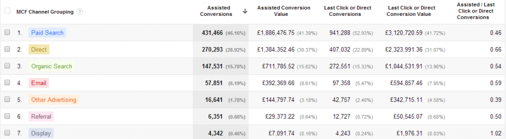
For example, take a look at the following information;
Assisted Conversion Summary Data within Google Analytics
It is clear to see that the Assisted Conversion Value is actually a significant amount, meaning that if you weren’t active in other areas then you would likely not have received this revenue or amount of enquiries. Most importantly you can then break this down into the various traffic sources so you can understand how they are contributing towards sales through your website.
Assisted Conversion Data within Google Analytics
Summary
Overall, there are a variety of ways you can use the features within Google Analytics to calculate a true return on your marketing spend. If you aren’t tracking your marketing activities, then quite simply you are spending aimlessly and are likely to be spending money without generating a return.
The key message to take away is that it is essential to be tracking all of your marketing activities to be able to make smarter data driven business decisions. Focus on marketing activities that are generating a return for your business and drop the areas that aren’t contributing.
Once you fully understand how your marketing activities are contributing towards increased enquiries and increased sales for your business this will transform the way you invest in marketing activities. All of this data allows you to calculate a true return on all of your marketing activities.
Spending your marketing budget is easy. Spending it on items that are delivering a return is a fine art. With tools as powerful as Google Analytics at our fingertips, surely every business is measuring the results from their marketing activities? Well, in our experience, even large and well established companies find it difficult to track marketing activities accurately.
What this means is that marketing budgets are often not spent as effectively as they could be. This would be fine if all businesses had an unlimited marketing budget, but this isn’t the case. Marketing budgets are always limited, which means that businesses need to be investing in marketing channels that are performing well for their business.
Throughout this blog post we will talk through the different ways you can track your marketing activities effectively which will mean you can make smarter data driven business decisions. Tracking marketing activities accurately means you can invest further in activities that are working well for your business and stop spending money on activities that aren’t generating a return.
All of the items we are going to talk about within this blog post are possible to track with ease through Google Analytics.
Set up Goals
What is the main goal you want website visitors to do? It is to purchase a product, enquire about the services or solutions you provide, or do you want them to download a guide from your website? Within Google Analytics you can set up a maximum of 20 goals within Google Analytics, which means that you can track an awful lot of data;
Set up Goals within Google Analytics
To track your marketing activities accurately this is absolutely essential to set up useful goals for your website. This can vary hugely between different websites based on what you are trying to achieve. Although have a think about both macro and micro goals on your website. What are the key things you want your website visitors to do?
Contact us
Request a call back
Follow you on social media channels
Purchase a product
Download a resource or guide
Find a local branch or store
Click and collect
Once you fully understand what you would like your website visitors to do, then you can start to track your marketing activities accurately. Quite simply, if you are paying for website visitors that aren’t working towards your key goals then maybe it is worth spending the marketing budget in areas that are working towards those goals instead.
Within Google Analytics, setting up goals couldn’t be easier with the many templates that are already available for you to customise for your individual website;
Goal Templates within Google Analytics
Use Goal Funnels
When you are setting up your goals above then you will be asked if you would like to use Goal Funnels. These are the specific steps that customers must go through before completing a goal. For example, if you are selling products online, then you will have multiple steps in the checkout process.
It is essential to set up the correct tracking for your purchasing funnel so you can understand how customers are behaving when they are completing this process. Below you can see an example for how this can be set up;
Goal Funnel Options within Google Analytics
Once you have configured this correctly you can easily visualise this information within Google Analytics. This will show you exactly how your website visitors are behaving and most importantly, where they are dropping out of the purchasing funnel. This is invaluable data that can provide insights into where improvements can be made to increase the number of people who complete their purchases.
Funnel Visualisation in Google Analytics
This data shows you the number of people who move on to the next step in the purchasing funnel and it will also show you the number of people who leave the purchasing funnel. More importantly, it will tell you where they went. Did they go to another page on the website for further information, or did they leave the website completely? This information can really help to understand your customer behaviours and look for ways of improving the user experience.
Ecommerce Tracking
If you are selling any products or services through your website, then setting up ecommerce tracking within Google Analytics is absolutely essential. The data that this provides means that you can easily see which products and services are the most popular, and most importantly, which traffic sources are leading to customers purchasing.
Understanding which traffic sources are working best for your business means that you can then readjust your marketing budgets towards the most profitable areas. Only through correct tracking is this possible. Below you can see some of the useful data that you will start to receive once you implement ecommerce tracking on your website and in Google Analytics;
Ecommerce Tracking within Google Analytics
Just as with goal tracking, the important point here is that once you fully understand which traffic sources and marketing activities are working towards increasing sales through your website, then you can start doing more of this. All of which is essential to fully understand how your marketing activities are performing.
Implementing ecommerce tracking is a little more involved than setting up goal tracking. Firstly you have to enable ecommerce tracking within Google Analytics then also implement additional tracking codes on your checkout completion page;
Ecommerce Setup within Google Analytics
To learn more about how ecommerce tracking can be set up, it is recommended that your website developer reads through the following guidelines from Google. To summarise the requirements, there needs to be additional information on the checkout complete page that contains all of the following information so that Google Analytics can pick this up and fire the data into the reporting platform;
Ecommerce Settings for Checkout Complete Page for Google Analytics
Call Tracking
One area that most businesses don’t realise is available is advanced call tracking tools which are designed to bridge the gap between your website analytics data and customers who call your office number. The reason why this is so important for a lot of businesses is because website visitors will often call the number on the website instead of completing a contact form.
What this means is that if you don’t have a call tracking solution in place, then you will be under reporting on the results. For example, if you ran a large pay per click advertising campaign and you started to receive a lot more phone enquiries, then this would be a challenge to monitor using only traditional website analytics. If this was the case, you would go back to monitor the performance of your recent campaign within Google Analytics and see that you received a lot of traffic to your website but very few people enquired using the contact form. You would likely mark this campaign as a poorly performing one and one that would guide your future investments in marketing activities down a different path. Where in fact, what has actually happened is that the campaign was a roaring success and generated a large amount of revenue, although it was all completed over the phone opposed to through the website.
Advanced call tracking solutions like this aren’t right for every business. Although if your business does do a lot of sales over the phone, then this really is something that you should be looking at. Purely to track all of your marketing activities accurately so you can calculate a true return on your marketing spend.
Assisted Conversions
Traditionally most businesses look at the results achieved from a marketing campaign on the basis of a ‘Last Click Attribution Model’, which simply means that the last traffic source that the website visitor used to arrive at your website is attributed to the success of that goal completion. For example, if a user visited your website first from organic search, then revisited a few days later through a link they found on another website, then revisited a few days after that via a pay per click advert on Google and made a purchase, this would mean that the pay per click advert is deemed to have been the traffic source that drove the sale.
Although what if this isn’t quite a true picture? What if the other two touch points were critical points within the purchasing journey and if they didn’t see these items, then they would have been less likely to purchase when they clicked on a pay per click advert?
Understanding the full customer purchasing journey is possible through the use of Assisted Conversions within Google Analytics. This powerful tool means that you can get a full and true picture of how your customers behave prior to purchasing your products and services.
For example, if you saw that people who read one of your travel guides or blog posts, then also read a review on a review website, were then more likely to purchase when they saw a pay per click advert, then you would be much more willing to invest in those other areas as you can attribute a value to these customers.
Let’s say those customers converted 20% higher than those who just arrived on a pay per click advert. This allows you to fully understand the key touch points that are contributing towards the customer enquiry or purchase. Knowing this means that
For example, take a look at the following information;
Assisted Conversion Summary Data within Google Analytics
It is clear to see that the Assisted Conversion Value is actually a significant amount, meaning that if you weren’t active in other areas then you would likely not have received this revenue or amount of enquiries. Most importantly you can then break this down into the various traffic sources so you can understand how they are contributing towards sales through your website.
Assisted Conversion Data within Google Analytics
Summary
Overall, there are a variety of ways you can use the features within Google Analytics to calculate a true return on your marketing spend. If you aren’t tracking your marketing activities, then quite simply you are spending aimlessly and are likely to be spending money without generating a return.
The key message to take away is that it is essential to be tracking all of your marketing activities to be able to make smarter data driven business decisions. Focus on marketing activities that are generating a return for your business and drop the areas that aren’t contributing.
Once you fully understand how your marketing activities are contributing towards increased enquiries and increased sales for your business this will transform the way you invest in marketing activities. All of this data allows you to calculate a true return on all of your marketing activities.
Within our daily work we use Excel an awful lot, so naturally we like to use Excel to its full potential using lots of exciting formulas. One of the major challenges within Excel is trying to use a VLOOKUP function within a VLOOKUP function. In summary, this isn’t possible. The reason this isn’t possible is due to the way the VLOOKUP function works. Let’s remind ourselves what the VLOOKUP function actually does;
What this means in basic terms is “find me a specific cell within a table of data where a certain criteria is met”. This is such a powerful function that can be used to speed up work in so many different ways. But we aren’t going to look at why this is so great here, we are going to look at the main limitation and most importantly how to get around this with more clever magical Excel formulas.
Solutions
The solution to this is quite a complex one and one that involves many different Excel formulas including;
=ROW()
=INDEX()
=SUMPRODUCT()
=MAX()
=ADDRESS()
=SUBSTITUTE()
=MATCH()
=CONCATENATE()
Throughout this blog post we’ll look at what each of these mean and how they can all be used in conjunction to perform a function what is essentially equivalent to a VLOOKUP within a VLOOKUP.
The Data
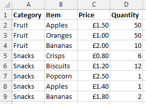
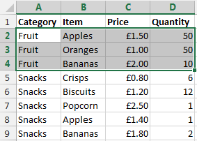
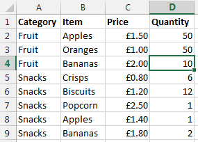
Before we jump into how to solve the problem of performing a VLOOKUP within a VLOOKUP, here is the data that we will be working with. Let’s assume that we have a large list of products which are associated with multiple different categories as can be seen below;
Data Sheet – Prices
You may be wondering why apples and bananas are classed as snacks in the data. Don’t worry about that. Just go with it. There are many different situations whereby you may be presented with this type of data so this is purely to illustrate the example in a simple way.
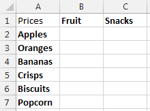
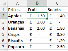
Now let’s say that you want to visualise this information a little easier. The above table of only 8 entries is reasonably straight forward. Although one example we’ve been recently working with had over 35,000 rows of data which was a little more challenging to view in this format and we wanted a simpler way of looking at this information within Excel. So let’s say we want to look at the data in the following way;
Data Sheet – Summary Prices
This is the data that we will be working with so you can clearly see how this technique can be implemented. To keep things easier to understand, these two pieces of data are kept on two separate sheets within the Excel worksheet.
Quick Answer
Looking for the quick answer to this complex formula? Then here is the answer;
You may be a little confused with the above, so this post will explain exactly what each part of this means and why it is contained within the rather large and complex formula above. Most importantly, you will be able to understand how to perform the equivalent of a VLOOKUP inside a VLOOKUP.
Steps
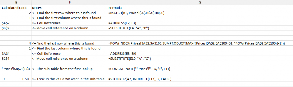
The individual steps within the above formula can be broken down into much smaller and easier to understand steps as can be seen below;
Steps for how to perform a VLOOKUP inside a VLOOKUP
Below we will talk through each of the above steps so you can understand why it is important.
Find the Sub-Table
Firstly if you are wanting to perform a VLOOKUP within a VLOOKUP then you need to find where the sub-table starts and ends. While you could manually enter this in for very small data sets, this is simply not practical for large data sets.
To perform this action we need to define search for the first and last occurrence of when ‘something’ is found. A note on this point, you will need to ensure that your lookup data, in this case the ‘Prices’ sheet, is ordered by the column you are looking up, in this case the ‘Category’ column. Since if this isn’t the case, then data will be included within this sub-table which shouldn’t be.
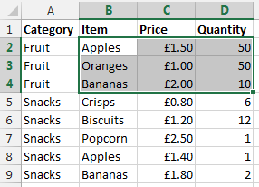
To do this, we need to find both the first occurrence and the last occurrence. What we are looking to achieve is identify the sub-table for ‘Fruit’ which can be seen below;
The sub-table we are looking for
Once this has been identified, then we can use the standard =VLOOKUP() function on this sub-table to find the data we would like.
Find the First Occurrence
There are a few different formulas included to find the first occurrence of data within a column which are outlined below.
=MATCH()
To find the first occurrence of ‘something’ within a range of data then we use the =MATCH() function. To remind ourselves of what the MATCH() function is, here is the official description from Microsoft;
The MATCH function searches for a specified item in a range of cells, and then returns the relative position of that item in the range. For example, if the range A1:A3 contains the values 5, 25, and 38, then the formula
=MATCH(25,A1:A3,0)
returns the number 2, because 25 is the second item in the range.
Use MATCH instead of one of the LOOKUP functions when you need the position of an item in a range instead of the item itself. For example, you might use the MATCH function to provide a value for the row_num argument of the INDEX function.
Looking back at our example, this translates into the formula;
=MATCH(B1, Prices!$A$1:$A$100, 0)
What this means is;
Find the contents of B1, which is ‘Fruit’ in our example
Within the range of data Prices!$A$1:$A$100
And make sure it matches exactly (0)
This has now found the first occurrence of this information within the column of data. Now we need to translate this into something that a VLOOKUP formula can use.
=ADDRESS()
The next bit we need to look at is turning the row & column numbers into an ‘Address’ which Excel can understand. To do this we simple create the formula;
=ADDRESS(E2, E3)
The =ADDRESS() function takes a Row Number and a Column Number and turns that into an Address. In this case, the row number is generated from the previous function, =MATCH() and the value of E3 in the example above is 1. We use 1 because for this we are only interested in starting on the first column of data. Once we know we are starting here we can always move the cells along accordingly.
In our example, this address at this point in the large formula is set to $A$2.
=SUBSTITUTE()
Now we know we have created an Address in the previous step which was within column 1, this is also the same as column A. This makes life easy for us as we know where this is. The next step is to nudge the sub-table over so the =VLOOKUP() function can easily lookup the data in the later step.
To do this, we simply nudge the starting Address over to the right by one column using the following formula;
=SUBSTITUTE(E4, “A”, “B”)
Where E4 is the cell which contains the Address from the previous step.
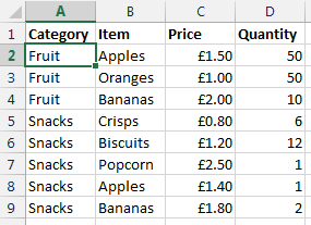
The cell that has been identified as part of this step is the first occurrence as can be seen below;
Find the first occurrence of data within the column
Now we want to nudge this over using the above function which will mean this item is now set to $B$2 which is the starting point of our sub-table.
Ok, so we now have the starting point for the sub-table for the VLOOKUP to use. We now need to calculate the end point so the sub-table can be used within the VLOOKUP.
Find the Last Occurrence
Finding the first occurrence of data in column is a lot easier than finding the last occurrence as you can see from the formula below that we need to do this;
=ROW() – Which takes a reference and calculates which row number this is on
=INDEX() – Which returns a value or the reference to a value from within a table or range.
=SUMPRODUCT() – This is used to tell Excel the calculations are an array and not an actual number
=MAX() – This is used to find the largest row number in the array where the lookup value occurs
=ROW() – This, as before, is pulling out the Row Number from the data retrieved
Unlike previously, it is not simple to break this out into sub-sections to explain the different points as the formulas don’t work when breaking them our separately due to the way the =SUMPRODUCT() function works. As such, I’ll talk through what each of the different parts of the formula mean and what they do.
This formula is identifying the last occurrence of the data that is in cell B1 within the range of data $A$2:$A$100, which in our example is ‘Fruit’. We then wrap this in the =INDEX() function to get the cell reference then wrapping this in the =ROW() function which will identify the row number where this data is found;
You may have spotted the -1 in the formula above. This is to ensure that the data is pulling back the correct row number. If this isn’t there, then you will notice that the data that is pulled back is a row below where you would expect.
To get a good understanding of the above part of the formula, then I’d recommend reading the fantastic guide over at Excel User.
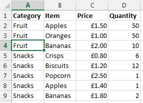
What we have achieved using the above combination of formulas can be seen below as the last occurrence of data in the column;
Find the last occurrence of data in the column
Once we have this data we then wrap this in an =ADDRESS() function then a =SUBSTITUTE() formula which first turns the result into an Address that Excel can understand, opposed to standard text, then moves the data over several columns from column A to column D. This is needed, since we will be creating a sub-table that includes several columns. In this case, 3 columns which are column B, C and D. If you are working with data with more columns, then you will need to replace the D with a higher column.
Move the column to the end so we can create a sub-table that contains all the required data
So now the end of the sub-table is set to $D$4 which means that we have a starting point and an end point for our sub-table which can be used in the =VLOOKUP() function as outlined below.
Lookup Data in the Sub-Table
Now we have the sub-table defined using all of the above formulas, we can use the standard =VLOOKUP() function once we have joined all of the above data together.
Create the lookup table
Now we have all of the above points, we need to create the lookup data using the standard =CONCATENATE() formula as can be seen below;
=CONCATENATE(“‘Prices’!”, E5, “:”, E11)
The data within E5 is the starting point of the sub-table, and the data within E11 is the end point within the sub-table. In our example, this gives us the answer of ‘Prices’!$B$2:$D$4.
Lookup data
Now we have the sub-table to lookup the data we want, we can simple use the standard =VLOOKUP() function to find the data that we require as follows;
=VLOOKUP(A2, INDIRECT(E13), 2, FALSE)
We wrap the concatenate function within the =INDIRECT() function so that the data is treated as a reference, opposed to text. The data within E13 is the result of all of the work previously in this post, I’ve just left this in here to make this easier to read and understand. For the full formula, this would be replaced with the individual parts. Now the data that is brought back is exactly what we want.
Sub-table of data based on initial criteria
What this final =VLOOKUP() function is doing is saying “find the value in A2 within the sub-table we have identified, then bring back the second column of data. So in our example, the long formula in column B1 is bringing back the data £1.50 as can be seen below;
Result of a VLOOKUP inside a VLOOKUP
Summary
So there you have it, how to perform the equivalent of a VLOOKUP within a VLOOKUP using a few different formulas within Excel. You may be a little scared of such a huge formula at first, but you will see that when you do need to use this, I would always recommend breaking this out into the different parts before trying to create one monolithic formula as you will be able to put this together much easier.
Also, in the formula below, you will notice that it is all wrapped in an =IFERROR() function which simply sets the data to 0 if nothing can be found. You can set this to whatever you like, I just chose 0 since this was about prices.
Ok, so this isn’t for the faint hearted. But for those advanced Excel users around I’m sure you will have come across times when you really needed to perform a VLOOKUP inside a VLOOKUP and found that after a long time researching how to do this online that it isn’t a simple task. So hopefully you can see the clear steps included above and this will help in the future. The beauty of the above formula is that you can now drag this into new rows and new columns without having to update anything, all thanks to the $ signs throughout the formula.
Within our daily work we use Excel an awful lot, so naturally we like to use Excel to its full potential using lots of exciting formulas. One of the major challenges within Excel is trying to use a VLOOKUP function within a VLOOKUP function. In summary, this isn’t possible. The reason this isn’t possible is due to the way the VLOOKUP function works. Let’s remind ourselves what the VLOOKUP function actually does;
What this means in basic terms is “find me a specific cell within a table of data where a certain criteria is met”. This is such a powerful function that can be used to speed up work in so many different ways. But we aren’t going to look at why this is so great here, we are going to look at the main limitation and most importantly how to get around this with more clever magical Excel formulas.
Solutions
The solution to this is quite a complex one and one that involves many different Excel formulas including;
=ROW()
=INDEX()
=SUMPRODUCT()
=MAX()
=ADDRESS()
=SUBSTITUTE()
=MATCH()
=CONCATENATE()
Throughout this blog post we’ll look at what each of these mean and how they can all be used in conjunction to perform a function what is essentially equivalent to a VLOOKUP within a VLOOKUP.
The Data
Before we jump into how to solve the problem of performing a VLOOKUP within a VLOOKUP, here is the data that we will be working with. Let’s assume that we have a large list of products which are associated with multiple different categories as can be seen below;
Data Sheet – Prices
You may be wondering why apples and bananas are classed as snacks in the data. Don’t worry about that. Just go with it. There are many different situations whereby you may be presented with this type of data so this is purely to illustrate the example in a simple way.
Now let’s say that you want to visualise this information a little easier. The above table of only 8 entries is reasonably straight forward. Although one example we’ve been recently working with had over 35,000 rows of data which was a little more challenging to view in this format and we wanted a simpler way of looking at this information within Excel. So let’s say we want to look at the data in the following way;
Data Sheet – Summary Prices
This is the data that we will be working with so you can clearly see how this technique can be implemented. To keep things easier to understand, these two pieces of data are kept on two separate sheets within the Excel worksheet.
Quick Answer
Looking for the quick answer to this complex formula? Then here is the answer;
You may be a little confused with the above, so this post will explain exactly what each part of this means and why it is contained within the rather large and complex formula above. Most importantly, you will be able to understand how to perform the equivalent of a VLOOKUP inside a VLOOKUP.
Steps
The individual steps within the above formula can be broken down into much smaller and easier to understand steps as can be seen below;
Steps for how to perform a VLOOKUP inside a VLOOKUP
Below we will talk through each of the above steps so you can understand why it is important.
Find the Sub-Table
Firstly if you are wanting to perform a VLOOKUP within a VLOOKUP then you need to find where the sub-table starts and ends. While you could manually enter this in for very small data sets, this is simply not practical for large data sets.
To perform this action we need to define search for the first and last occurrence of when ‘something’ is found. A note on this point, you will need to ensure that your lookup data, in this case the ‘Prices’ sheet, is ordered by the column you are looking up, in this case the ‘Category’ column. Since if this isn’t the case, then data will be included within this sub-table which shouldn’t be.
To do this, we need to find both the first occurrence and the last occurrence. What we are looking to achieve is identify the sub-table for ‘Fruit’ which can be seen below;
The sub-table we are looking for
Once this has been identified, then we can use the standard =VLOOKUP() function on this sub-table to find the data we would like.
Find the First Occurrence
There are a few different formulas included to find the first occurrence of data within a column which are outlined below.
=MATCH()
To find the first occurrence of ‘something’ within a range of data then we use the =MATCH() function. To remind ourselves of what the MATCH() function is, here is the official description from Microsoft;
The MATCH function searches for a specified item in a range of cells, and then returns the relative position of that item in the range. For example, if the range A1:A3 contains the values 5, 25, and 38, then the formula
=MATCH(25,A1:A3,0)
returns the number 2, because 25 is the second item in the range.
Use MATCH instead of one of the LOOKUP functions when you need the position of an item in a range instead of the item itself. For example, you might use the MATCH function to provide a value for the row_num argument of the INDEX function.
Looking back at our example, this translates into the formula;
=MATCH(B1, Prices!$A$1:$A$100, 0)
What this means is;
Find the contents of B1, which is ‘Fruit’ in our example
Within the range of data Prices!$A$1:$A$100
And make sure it matches exactly (0)
This has now found the first occurrence of this information within the column of data. Now we need to translate this into something that a VLOOKUP formula can use.
=ADDRESS()
The next bit we need to look at is turning the row & column numbers into an ‘Address’ which Excel can understand. To do this we simple create the formula;
=ADDRESS(E2, E3)
The =ADDRESS() function takes a Row Number and a Column Number and turns that into an Address. In this case, the row number is generated from the previous function, =MATCH() and the value of E3 in the example above is 1. We use 1 because for this we are only interested in starting on the first column of data. Once we know we are starting here we can always move the cells along accordingly.
In our example, this address at this point in the large formula is set to $A$2.
=SUBSTITUTE()
Now we know we have created an Address in the previous step which was within column 1, this is also the same as column A. This makes life easy for us as we know where this is. The next step is to nudge the sub-table over so the =VLOOKUP() function can easily lookup the data in the later step.
To do this, we simply nudge the starting Address over to the right by one column using the following formula;
=SUBSTITUTE(E4, “A”, “B”)
Where E4 is the cell which contains the Address from the previous step.
The cell that has been identified as part of this step is the first occurrence as can be seen below;
Find the first occurrence of data within the column
Now we want to nudge this over using the above function which will mean this item is now set to $B$2 which is the starting point of our sub-table.
Ok, so we now have the starting point for the sub-table for the VLOOKUP to use. We now need to calculate the end point so the sub-table can be used within the VLOOKUP.
Find the Last Occurrence
Finding the first occurrence of data in column is a lot easier than finding the last occurrence as you can see from the formula below that we need to do this;
=ROW() – Which takes a reference and calculates which row number this is on
=INDEX() – Which returns a value or the reference to a value from within a table or range.
=SUMPRODUCT() – This is used to tell Excel the calculations are an array and not an actual number
=MAX() – This is used to find the largest row number in the array where the lookup value occurs
=ROW() – This, as before, is pulling out the Row Number from the data retrieved
Unlike previously, it is not simple to break this out into sub-sections to explain the different points as the formulas don’t work when breaking them our separately due to the way the =SUMPRODUCT() function works. As such, I’ll talk through what each of the different parts of the formula mean and what they do.
This formula is identifying the last occurrence of the data that is in cell B1 within the range of data $A$2:$A$100, which in our example is ‘Fruit’. We then wrap this in the =INDEX() function to get the cell reference then wrapping this in the =ROW() function which will identify the row number where this data is found;
You may have spotted the -1 in the formula above. This is to ensure that the data is pulling back the correct row number. If this isn’t there, then you will notice that the data that is pulled back is a row below where you would expect.
To get a good understanding of the above part of the formula, then I’d recommend reading the fantastic guide over at Excel User.
What we have achieved using the above combination of formulas can be seen below as the last occurrence of data in the column;
Find the last occurrence of data in the column
Once we have this data we then wrap this in an =ADDRESS() function then a =SUBSTITUTE() formula which first turns the result into an Address that Excel can understand, opposed to standard text, then moves the data over several columns from column A to column D. This is needed, since we will be creating a sub-table that includes several columns. In this case, 3 columns which are column B, C and D. If you are working with data with more columns, then you will need to replace the D with a higher column.
Move the column to the end so we can create a sub-table that contains all the required data
So now the end of the sub-table is set to $D$4 which means that we have a starting point and an end point for our sub-table which can be used in the =VLOOKUP() function as outlined below.
Lookup Data in the Sub-Table
Now we have the sub-table defined using all of the above formulas, we can use the standard =VLOOKUP() function once we have joined all of the above data together.
Create the lookup table
Now we have all of the above points, we need to create the lookup data using the standard =CONCATENATE() formula as can be seen below;
=CONCATENATE(“‘Prices’!”, E5, “:”, E11)
The data within E5 is the starting point of the sub-table, and the data within E11 is the end point within the sub-table. In our example, this gives us the answer of ‘Prices’!$B$2:$D$4.
Lookup data
Now we have the sub-table to lookup the data we want, we can simple use the standard =VLOOKUP() function to find the data that we require as follows;
=VLOOKUP(A2, INDIRECT(E13), 2, FALSE)
We wrap the concatenate function within the =INDIRECT() function so that the data is treated as a reference, opposed to text. The data within E13 is the result of all of the work previously in this post, I’ve just left this in here to make this easier to read and understand. For the full formula, this would be replaced with the individual parts. Now the data that is brought back is exactly what we want.
Sub-table of data based on initial criteria
What this final =VLOOKUP() function is doing is saying “find the value in A2 within the sub-table we have identified, then bring back the second column of data. So in our example, the long formula in column B1 is bringing back the data £1.50 as can be seen below;
Result of a VLOOKUP inside a VLOOKUP
Summary
So there you have it, how to perform the equivalent of a VLOOKUP within a VLOOKUP using a few different formulas within Excel. You may be a little scared of such a huge formula at first, but you will see that when you do need to use this, I would always recommend breaking this out into the different parts before trying to create one monolithic formula as you will be able to put this together much easier.
Also, in the formula below, you will notice that it is all wrapped in an =IFERROR() function which simply sets the data to 0 if nothing can be found. You can set this to whatever you like, I just chose 0 since this was about prices.
Ok, so this isn’t for the faint hearted. But for those advanced Excel users around I’m sure you will have come across times when you really needed to perform a VLOOKUP inside a VLOOKUP and found that after a long time researching how to do this online that it isn’t a simple task. So hopefully you can see the clear steps included above and this will help in the future. The beauty of the above formula is that you can now drag this into new rows and new columns without having to update anything, all thanks to the $ signs throughout the formula.