Within our daily work we use Excel an awful lot, so naturally we like to use Excel to its full potential using lots of exciting formulas. One of the major challenges within Excel is trying to use a VLOOKUP function within a VLOOKUP function. In summary, this isn’t possible. The reason this isn’t possible is due to the way the VLOOKUP function works. Let’s remind ourselves what the VLOOKUP function actually does;

=VLOOKUP(lookup_value,table_array,col_index_num,range_lookup)

What this means in basic terms is “find me a specific cell within a table of data where a certain criteria is met”. This is such a powerful function that can be used to speed up work in so many different ways. But we aren’t going to look at why this is so great here, we are going to look at the main limitation and most importantly how to get around this with more clever magical Excel formulas.

Solutions

The solution to this is quite a complex one and one that involves many different Excel formulas including;

• =ROW()
• =INDEX()
• =SUMPRODUCT()
• =MAX()
• =ADDRESS()
• =SUBSTITUTE()
• =MATCH()
• =CONCATENATE()

Throughout this blog post we’ll look at what each of these mean and how they can all be used in conjunction to perform a function what is essentially equivalent to a VLOOKUP within a VLOOKUP.

The Data

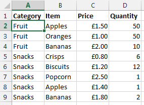
Before we jump into how to solve the problem of performing a VLOOKUP within a VLOOKUP, here is the data that we will be working with. Let’s assume that we have a large list of products which are associated with multiple different categories as can be seen below;

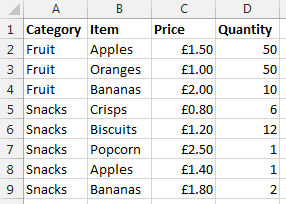
Data Sheet – Prices

You may be wondering why apples and bananas are classed as snacks in the data. Don’t worry about that. Just go with it. There are many different situations whereby you may be presented with this type of data so this is purely to illustrate the example in a simple way.

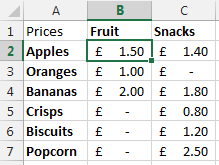
Now let’s say that you want to visualise this information a little easier. The above table of only 8 entries is reasonably straight forward. Although one example we’ve been recently working with had over 35,000 rows of data which was a little more challenging to view in this format and we wanted a simpler way of looking at this information within Excel. So let’s say we want to look at the data in the following way;

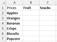
Data Sheet – Summary Prices

This is the data that we will be working with so you can clearly see how this technique can be implemented. To keep things easier to understand, these two pieces of data are kept on two separate sheets within the Excel worksheet.

Quick Answer

Looking for the quick answer to this complex formula? Then here is the answer;

=IFERROR(VLOOKUP($A2, INDIRECT(CONCATENATE(“‘Prices’!”, SUBSTITUTE(ADDRESS(MATCH(B$1, Prices!$A$1:$A$100, 0), 1), “A”, “B”), “:”, SUBSTITUTE(ADDRESS(ROW(INDEX(Prices!$A$2:$A$100,SUMPRODUCT(MAX((Prices!$A$2:$A$100=B$1)*ROW(Prices!$A$2:$A$100))-1))), 1), “A”, “D”))), 2, FALSE), 0)

You may be a little confused with the above, so this post will explain exactly what each part of this means and why it is contained within the rather large and complex formula above. Most importantly, you will be able to understand how to perform the equivalent of a VLOOKUP inside a VLOOKUP.

Steps

The individual steps within the above formula can be broken down into much smaller and easier to understand steps as can be seen below;

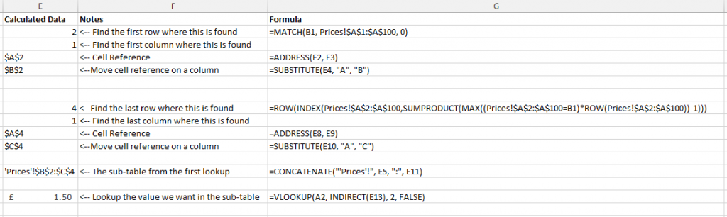
Steps for how to perform a VLOOKUP inside a VLOOKUP

Below we will talk through each of the above steps so you can understand why it is important.

Find the Sub-Table

Firstly if you are wanting to perform a VLOOKUP within a VLOOKUP then you need to find where the sub-table starts and ends. While you could manually enter this in for very small data sets, this is simply not practical for large data sets.

To perform this action we need to define search for the first and last occurrence of when ‘something’ is found. A note on this point, you will need to ensure that your lookup data, in this case the ‘Prices’ sheet, is ordered by the column you are looking up, in this case the ‘Category’ column. Since if this isn’t the case, then data will be included within this sub-table which shouldn’t be.

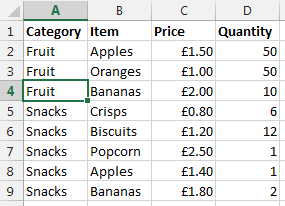
To do this, we need to find both the first occurrence and the last occurrence. What we are looking to achieve is identify the sub-table for ‘Fruit’ which can be seen below;

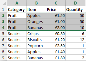
The sub-table we are looking for

Once this has been identified, then we can use the standard =VLOOKUP() function on this sub-table to find the data we would like.

Find the First Occurrence

There are a few different formulas included to find the first occurrence of data within a column which are outlined below.

=MATCH()

To find the first occurrence of ‘something’ within a range of data then we use the =MATCH() function. To remind ourselves of what the MATCH() function is, here is the official description from Microsoft;

The MATCH function searches for a specified item in a range of cells, and then returns the relative position of that item in the range. For example, if the range A1:A3 contains the values 5, 25, and 38, then the formula

=MATCH(25,A1:A3,0)

returns the number 2, because 25 is the second item in the range.

Use MATCH instead of one of the LOOKUP functions when you need the position of an item in a range instead of the item itself. For example, you might use the MATCH function to provide a value for the row_num argument of the INDEX function.

MATCH(lookup_value, lookup_array, [match_type])

Source

Looking back at our example, this translates into the formula;

=MATCH(B1, Prices!$A$1:$A$100, 0)

What this means is;

• Find the contents of B1, which is ‘Fruit’ in our example
• Within the range of data Prices!$A$1:$A$100
• And make sure it matches exactly (0)

This has now found the first occurrence of this information within the column of data. Now we need to translate this into something that a VLOOKUP formula can use.

=ADDRESS()

The next bit we need to look at is turning the row & column numbers into an ‘Address’ which Excel can understand. To do this we simple create the formula;

=ADDRESS(E2, E3)

The =ADDRESS() function takes a Row Number and a Column Number and turns that into an Address. In this case, the row number is generated from the previous function, =MATCH() and the value of E3 in the example above is 1. We use 1 because for this we are only interested in starting on the first column of data. Once we know we are starting here we can always move the cells along accordingly.

In our example, this address at this point in the large formula is set to $A$2.

=SUBSTITUTE()

Now we know we have created an Address in the previous step which was within column 1, this is also the same as column A. This makes life easy for us as we know where this is. The next step is to nudge the sub-table over so the =VLOOKUP() function can easily lookup the data in the later step.

To do this, we simply nudge the starting Address over to the right by one column using the following formula;

=SUBSTITUTE(E4, “A”, “B”)

Where E4 is the cell which contains the Address from the previous step.

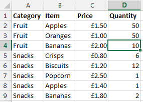
The cell that has been identified as part of this step is the first occurrence as can be seen below;

Find the first occurrence of data within the column

Now we want to nudge this over using the above function which will mean this item is now set to $B$2 which is the starting point of our sub-table.

Ok, so we now have the starting point for the sub-table for the VLOOKUP to use. We now need to calculate the end point so the sub-table can be used within the VLOOKUP.

Find the Last Occurrence

Finding the first occurrence of data in column is a lot easier than finding the last occurrence as you can see from the formula below that we need to do this;

=ROW(INDEX(Prices!$A$2:$A$100,SUMPRODUCT(MAX((Prices!$A$2:$A$100=B1)*ROW(Prices!$A$2:$A$100))-1)))

The key functions we need here are;

• =ROW() – Which takes a reference and calculates which row number this is on
• =INDEX() – Which returns a value or the reference to a value from within a table or range.
• =SUMPRODUCT() – This is used to tell Excel the calculations are an array and not an actual number
• =MAX() – This is used to find the largest row number in the array where the lookup value occurs
• =ROW() – This, as before, is pulling out the Row Number from the data retrieved

Unlike previously, it is not simple to break this out into sub-sections to explain the different points as the formulas don’t work when breaking them our separately due to the way the =SUMPRODUCT() function works. As such, I’ll talk through what each of the different parts of the formula mean and what they do.

=SUMPRODUCT(MAX((Prices!$A$2:$A$100=B1)*ROW(Prices!$A$2:$A$100))-1)

This formula is identifying the last occurrence of the data that is in cell B1 within the range of data $A$2:$A$100, which in our example is ‘Fruit’. We then wrap this in the =INDEX() function to get the cell reference then wrapping this in the =ROW() function which will identify the row number where this data is found;

=ROW(INDEX(Prices!$A$2:$A$100, SUMPRODUCT(MAX((Prices!$A$2:$A$100=B1)*ROW(Prices!$A$2:$A$100))-1)))

You may have spotted the -1 in the formula above. This is to ensure that the data is pulling back the correct row number. If this isn’t there, then you will notice that the data that is pulled back is a row below where you would expect.

To get a good understanding of the above part of the formula, then I’d recommend reading the fantastic guide over at Excel User.

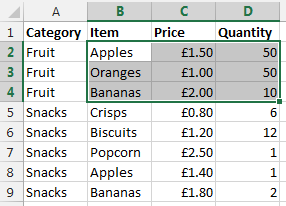
What we have achieved using the above combination of formulas can be seen below as the last occurrence of data in the column;

Find the last occurrence of data in the column

Once we have this data we then wrap this in an =ADDRESS() function then a =SUBSTITUTE() formula which first turns the result into an Address that Excel can understand, opposed to standard text, then moves the data over several columns from column A to column D. This is needed, since we will be creating a sub-table that includes several columns. In this case, 3 columns which are column B, C and D. If you are working with data with more columns, then you will need to replace the D with a higher column.

SUBSTITUTE(ADDRESS(ROW(INDEX(Prices!$A$2:$A$100,SUMPRODUCT(MAX((Prices!$A$2:$A$100=B$1)*ROW(Prices!$A$2:$A$100))-1))), 1), “A”, “D”)))

Move the column to the end so we can create a sub-table that contains all the required data

So now the end of the sub-table is set to $D$4 which means that we have a starting point and an end point for our sub-table which can be used in the =VLOOKUP() function as outlined below.

Lookup Data in the Sub-Table

Now we have the sub-table defined using all of the above formulas, we can use the standard =VLOOKUP() function once we have joined all of the above data together.

Create the lookup table

Now we have all of the above points, we need to create the lookup data using the standard =CONCATENATE() formula as can be seen below;

=CONCATENATE(“‘Prices’!”, E5, “:”, E11)

The data within E5 is the starting point of the sub-table, and the data within E11 is the end point within the sub-table. In our example, this gives us the answer of ‘Prices’!$B$2:$D$4.

Lookup data

Now we have the sub-table to lookup the data we want, we can simple use the standard =VLOOKUP() function to find the data that we require as follows;

=VLOOKUP(A2, INDIRECT(E13), 2, FALSE)

We wrap the concatenate function within the =INDIRECT() function so that the data is treated as a reference, opposed to text. The data within E13 is the result of all of the work previously in this post, I’ve just left this in here to make this easier to read and understand. For the full formula, this would be replaced with the individual parts. Now the data that is brought back is exactly what we want.

Sub-table of data based on initial criteria

What this final =VLOOKUP() function is doing is saying “find the value in A2 within the sub-table we have identified, then  bring back the second column of data. So in our example, the long formula in column B1 is bringing back the data £1.50 as can be seen below;

Result of a VLOOKUP inside a VLOOKUP

Summary

So there you have it, how to perform the equivalent of a VLOOKUP within a VLOOKUP using a few different formulas within Excel. You may be a little scared of such a huge formula at first, but you will see that when you do need to use this, I would always recommend breaking this out into the different parts before trying to create one monolithic formula as you will be able to put this together much easier.

Also, in the formula below, you will notice that it is all wrapped in an =IFERROR() function which simply sets the data to 0 if nothing can be found. You can set this to whatever you like, I just chose 0 since this was about prices.

=IFERROR(VLOOKUP($A2, INDIRECT(CONCATENATE(“‘Prices’!”, SUBSTITUTE(ADDRESS(MATCH(B$1, Prices!$A$1:$A$100, 0), 1), “A”, “B”), “:”, SUBSTITUTE(ADDRESS(ROW(INDEX(Prices!$A$2:$A$100,SUMPRODUCT(MAX((Prices!$A$2:$A$100=B$1)*ROW(Prices!$A$2:$A$100))-1))), 1), “A”, “D”))), 2, FALSE), 0)

=IFERROR(VLOOKUP({Main-Lookup-Value}, INDIRECT(CONCATENATE(“‘{Sheet}‘!”, SUBSTITUTE(ADDRESS(MATCH({Sub-Table-Lookup-Value-First-Occurrence}, {Sheet}!{Sub-Table-Lookup-Range}, 0), 1), “A”, “B”), “:”, SUBSTITUTE(ADDRESS(ROW(INDEX({Sheet}!{Sub-Table-Lookup-Range},SUMPRODUCT(MAX(({Sheet}!{Sub-Table-Lookup-Range}={Sub-Table-Lookup-Value-Last-Occurrence})*ROW({Sheet}!{Sub-Table-Lookup-Range}))-1))), 1), “A”, “{Column-Letter-For-End-Of-Table}“))), 2, FALSE), 0)

Simple really!

Ok, so this isn’t for the faint hearted. But for those advanced Excel users around I’m sure you will have come across times when you really needed to perform a VLOOKUP inside a VLOOKUP and found that after a long time researching how to do this online that it isn’t a simple task. So hopefully you can see the clear steps included above and this will help in the future. The beauty of the above formula is that you can now drag this into new rows and new columns without having to update anything, all thanks to the $ signs throughout the formula.

The following two tabs change content below.

• Bio
• Latest Posts

Michael Cropper

Founder & Managing Director at Contrado Digital Ltd

Michael has been running Contrado Digital for over 10 years and has over 15 years experience working across the full range of disciplines including IT, Tech, Software Development, Digital Marketing, Analytics, SaaS, Startups, Organisational and Systems Thinking, DevOps, Project Management, Multi-Cloud, Digital and Technology Innovation and always with a business and commercial focus. He has a wealth of experience working with national and multi-national brands in a wide range of industries, across a wide range of specialisms, helping them achieve awesome results. Digital transformation, performance and collaboration are at the heart of everything Michael does.

Latest posts by Michael Cropper (see all)

• How to Setup Your Local Development Environment for Java Using Apache NetBeans and Apache Tomcat - December 1, 2023
• MySQL Recursive Queries – MySQL While Loops – Fill Zero Sum Dates Between Dates - October 6, 2023
• Has Stack Overflow Really Improved their Community Problems in 5 Years? - May 3, 2023