by Michael Cropper | Dec 14, 2012 | Developer |
XPathOnURL is an amazing function within the amazing SEO Tools plugin for Excel that can scrape specific pieces of content that you need when entering in a URL and the XPath of the content that you want to retrieve. This post isn’t going to be a quite to XPathOnURL, nor is it going to be a guide to XPath – instead what it is looking at is a way to retrieve multiple pieces of data when using XPathOnURL. If you are interested in playing around with XPath then download the XPath Helper plugin for Google Chrome that will help you get the XPath of the items you want to scrape.
By default the XPathOnURL function within the SEO Tools plugin only brings back the first occurrence of the item within the DOM (Document Object Model – i.e the HTML of the page..). As an example lets take my blogroll;

When using the XPath Helper plugin for Google Chrome, and tweaking the XPath a little to get what I need, you can see that the XPath present is showing that there are four links present within the blogroll;

All sounds good right. Well not quite, since when you copy this XPath into the XPathOnURL formula as part of SEO Tools then you will only get back the first URL instead of all four of them. Note, you cannot simply copy the exact XPath as shown in the screenshot above since you need to do something slightly different to scrape the HREF attribute using XPathOnURL – luckily I wrote a blog post just about that a while ago!
For the purpose of this blog post, I will use the XPath version for use with XPathOnURL without further explanation about that – read the previous blog post if this doesn’t make sense.
Anyways, back to the point. So when trying to scrape all four of the blogroll links using XPathOnURL you would think it would be as simple as entering the correct formula right? Unfortunately not. Blow is what happens when you try and do this;

While it is useful to get something back, it isn’t quite what I wanted. Instead I wanted all of the links to come back with this query which is more useful than just the first one. Depending on what you are scraping this can be a bit of a pain if there are quite a few pieces of content you want to scrape.
Luckily there is another function within SEO Tools for Excel which is the StringJoin(“,”, “……”) function (information) which helpfully joins together data and separates them by whatever you want – in this case, I have chosen a comma to separate the results by.
How this function can be used in conjunction with XPathOnURL is that you simple wrap it around the previous formula shown above and tell Excel to separate the results using a comma as seen in the example below;

This is a little more useful! So now we have all of the scraped data that we need. From here you can easily count the number of occurrences of a comma in the cell which will tell you how many pieces of data you have scraped. Or alternatively you could use the handy text to columns tool that is built into Excel by default to split out the data into separate columns (if you would prefer it in Rows instead then use the Transposetool)
On a small scale like this it is easy enough to do this manually. But recently I had need to do this for around 500 URLs each with an unknown amount of ‘bits’ on that I needed to count. Life is too short to be doing that kind of stuff manually so found a nice quick way of doing this using a few formulas and a bit of Excel magic. It turned out that the results were over 6500 ‘bits’ which would have taken me an awful long time to count manually!
So hopefully this formula can help save you some time when trying to return multiple nodes using XPathOnURL.
As a final note, as I was writing this post on another computer (and creating the formulas and screenshots for this post etc.), I noticed that the latest version of SEO Tools for Excel actually does this out of the box automatically. So if you don’t want to be doing all of this work manually then maybe it is just easier to upgrade to the latest version of the plugin  Below is what it looks like when using the latest version with all of the pieces of data you have scraped separated by a semi-colon ;

Thought I would carry on writing the post anyway as it would have saved me a bit of time earlier if I came across this post as I didn’t realise I wasn’t running the latest version!
by Michael Cropper | Oct 14, 2012 | Developer |
The joys of XPath and SEO Tools for Excel. Here we are going to talk through how to scrape the HREF attribute using the =XPathOnURLfunction as this is often needed when you want to scrape the actual links from a website which match a certain criteria.
If you just want the quick answer, here is how you do it;
=XPathOnURL(“http://www.example.com”, “//a”, “href”)
Well something like that anyways, as it depends on the actual XPath you need to use to get the actual links you need. One thing to note about the XPathOnURL function is that it doesn’t work quite the same as standard XPath but this will be explained a little later.
Firstly if you want to scrape the HREF attribute then you may actually be able to do this much quicker using the Google Chrome plugin calledXPath Helper, but that isn’t always the case.
Example
I came across an example recently when I needed to scrape one HREF attribute on around 100 pages, so the XPath Helper plugin wouldn’t quite do it. Below shows the setup that I was working with whereby there was a lot of pages where I needed to scrape some data, particularly one specific HREF attribute as is shown in the example below;

In the example above I am wanting to scrape a link to an image file which just happens to be within the first Div on the page (in this fictitious example!).
Normally if I wanted to do this via standard XPath then I would use the XPath of: //div/a[@href] – which is saying “get the HREF attribute which is contained within an A tag which is contained within a DIV tag.
When using the XPathOnURL function within SEO Tools then this doesn’t quite work in the same way. Instead if you want to pull back an attribute instead of the content between the opening and closing tags, then you need to add the extra parameter within the function which is: , “href” – which is telling the function to pull back the HREF attribute instead.
I am sure that you will come across a need for this at some point – especially if doing a lot of scraping!
That is all of the explanation I am going to do here. Go and give it a go yourself if you ever need to scrape the HREF attribute using XPathOnURL 
by Michael Cropper | Aug 14, 2012 | Developer |
If you have ever used the VLOOKUP function within Excel before and tried the “Approximate Match” type then you will have realised that this is about as useful as a chocolate tea cup. Below shows how you can easily and quickly perform a VLOOKUP using a partial match on the look up value.
For those of you who just want the answer quickly then here is the formula to VLOOKUP on a partial match;
=VLOOKUP(CONCATENATE(“*”, A2, “*”), ‘Tab2’!$A$2:$A$100, 1, FALSE)
So what does all of that mean?
The VLOOKUP formula is described as
=VLOOKUP({lookup this value or string}, {within this range of data}, {bring back this column number}, {TRUE (approximate match) or FALSE (exact match)}
So as an example if you have the following data to play around with;
Tab 1
Cell A2: “Jim”
Tab 2
Cell A2: “Jim Bob”
Then if you run the formula “=VLOOKUP(A2, ‘Tab2’!$A$2:$A$100), 1, FALSE)” which is aiming to find the string “Jim” within the range of data in the second tab with an exact match. Since this doesn’t exist within the range of data in its exact form then this will return “#N/A” as the result since it cannot be found.
If you try the exact same method but use a partial match instead then you could get any number of results returned depending on the size of the range of data you are working with. I am not going to cover the details about why the partial match on VLOOKUPs using “True” as the match type is a waste of time in this blog post, just trust me – it is awful, I have never found a reason why this would exist (I’m sure they may be some reason, I just haven’t ever found a use for it!).
VLOOKUP Partial Match
So if you want to look up a partial match which doesn’t use the “Approximate Match” type then you need to do a bit of clever excel magic.
In this instance the * character represents a wildcard which means that when Excel is looking up the value it uses the lookup for a partial match yet still follows the strict criteria of the “Exact Match” type of the VLOOKUP formula.
Let me explain that in a little more detail.
So here is the original formula again;
=VLOOKUP(CONCATENATE(“*”, A2, “*”), ‘Tab2’!$A$2:$A$100, 1, FALSE)
What this formula is saying is as follows;
- CONCATENATE(“*”, A2, “*”): Add an * at the start and end of the value which is being looked up, in this case cell A2
- =VLOOKUP(…{above formula}…): Look up this value
- ‘Tab2’!$A$2:$A$100: Lookup the original value within this range of data
- 1: Bring back this column of data when the item is found
- FALSE: Still use the “Exact Match” type as part of the VLOOKUP function
So it really is as simple as that to look up a partial match on a row of data
Alternative Uses
Alternative uses when you want to perform a partial match look up could be if you wanted to count the number of times where a certain piece of text was occurring within a range of data as follows;
Tab 1
A2: Jim Bob
A3: Jimmy
A4: Bob
A5: Jimmy Mallet
Then if you performed the following formula on the above range of data;
=IF(COUNTIF(A2:A5,CONCATENATE(“*”, “Jim”, “*”))>0,”Yes”,”No”)
Then this would count the number of cells which contain the word “Jim” within the range of data, in this case 3. In the example above it simply outputs a “Yes” or a “No” if there is at least one occurrence of the word within the range of data, although if you would like the exact figure then you can simply strip that part of the formula out which would become;
=COUNTIF(A1:A4,CONCATENATE(“*”, “Jim”, “*”))
A few nice quick Excel tips to help with looking up values in Excel using partial matches.
Previous Comments
by Michael Cropper | Aug 14, 2012 | SEO |
A large part of SEO is all about link building, you don’t need me to tell you that. What is important though is not just the changes in rankings which are happening due to the link building but also the amount of referral traffic which is coming through from this work.
If your links aren’t generating traffic then I would begin to question the long term success those types of links are having on your website, rankings and brand.
Below outlines a quick and simple step by step process to quickly assess how effective your link building techniques have been in generating traffic to your website.
Step 1: Download all referral traffic from Google Analytics
Go to Google Analytics –> Traffic Sources –> Sources –> Referrals
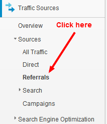
Then view the maximum amount of rows, 500 by using the filter at the bottom of the screen.

Then export all of this data into a CSV file which can easily be opened later in Excel. Click on Export –> CSV at the top of the screen as shown in the screenshot below
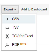
Step 2 – Combine Links Data with Rererral traffic
The next step is to open up the file you have just download and re-save this as a normal Excel file as we will be adding in some more tabs, data and look-ups which standard CSV files aren’t designed to handle.
Once you have done this do the following;
- Rename the first tab to ‘Google Analytics Referral Data’
- Create a second tab called ‘Links Built’
This will help when doing the cool excel magic a little later.
Now you need to simply add into the tab ‘Links Built’ (you guessed it!) all of the links you have built!
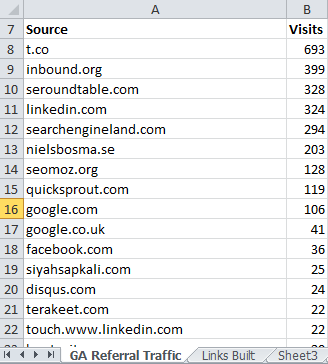
Below is a screenshot of some of the referral traffic to my website;
Below is a screenshot of some of the links which I have built to my site by shamelessly self promoting my content;
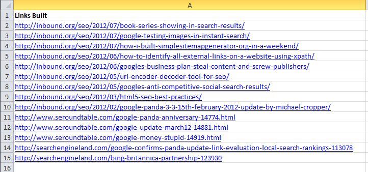
The links in the above screenshot are just a small sample I have scraped together for this blog post, I don’t actually keep track of this for my own blog – I have got much better things to do with my life  For people building links in competitive industries and on larger websites then you will likely have lists which go into the hundreds or thousands, so this method can really save some time for you.
So now you have all of the link and referral data within one Excel file which you can then do some cool Excel magic on.
Step 3 – Do Cool Excel Magic
Now you want to find out how many visitors the link building has resulted in. As mentioned previously, if you are just building links for the SEO value and not for traffic is this really going to be a good long term SEO strategy…?
The next step here is to add an extra column next to the list of referral traffic to see if this referral traffic was from the effort you put into link building;

If you want to copy and paste the formula then it is;
=IF(COUNTIF(‘Links Built’!$A$2:$A$100,CONCATENATE(“*”, A8, “*”))>0,”Yes”,”No”)
The formula may look a little scary but all it is essentially saying is: “See if this domain in A8 is contained within the list of links which I have built”. For a full guide on what this means take a look through the blog post explaining this in detail, How to VLOOKUP Using Partial Match
The different parts of the formula are saying;
- Count the range of cells, A2:A100 if….
- The cell contains a partial match on cell A8
- If there is a match, then put “Yes” in the cell
- If not, then put “No” in the cell
Now simply drag this formula down through to all of your referral traffic to see if this was from a link which was built or not.
Note, this check is only looking at the domain name and not page specific. So if you built a link on www.example.com/page1.html which drove 0 visits and you got an organic link on www.example.com/page2.html which drove 100 visits then all of this traffic would be attributed towards the link building work which you have done – which isn’t correct in this example.
By default Google Analytics doesn’t display the full referral path, but only domain name. It is possible to set up an additional profile within Google Analytics, to get the full URL for referrals then follow the guide in the link. One thing to note is that Google Analytics profiles only show data from the date they were set up, so you cannot see historical data with this method. Although if you get it set up now then you can begin to get more accurate data in the future.
Second note, the formula described above can also be run as aVLOOKUP if you need to pull the data back into this tab by simply editing the formula as follows (although this method will only bring back the first occurrence of the domain name mentioned, unless you have the full referral path within your analytics profile);
=VLOOKUP(CONCATENATE(“*”, A8, “*”), ‘Links Built’!$A$2:$A$100, 1, FALSE)
Step 4 – Analyse the Data
Now you will have ended up with a list of Yes/No’s which will tell you if you have built the link for this traffic source. Below is an example of how this can look after you have filtered by all of the “Yes”;

As you can see from three domains listed above, these have driven over 1000 visits to my blog in a short period of time. Are these good for SEO? Well traditionally you may argue that the links are no followed so they don’t offer any value. Personally I would rather have a no followed link which drives actual traffic and real people to my website instead of a followed link which doesn’t drive any traffic at all.
I would suggest running reports like this on a regular basis to continually assess if the work you are doing is actually driving real users to your website and not just building links for the pure PageRank benefit of the link. If all of your links have driven 0 traffic to your website in the past X months then I would begin to ask yourself if what you are doing is going to be having real long term results for your website.
If you also track the type of website where you have been building links such as, guest blog post, infographics, directories etc. then you can quickly assess which type of links are or aren’t driving traffic to your website which can help gain further insights into what is working from a traffic point.
by Michael Cropper | Jul 14, 2012 | Developer |
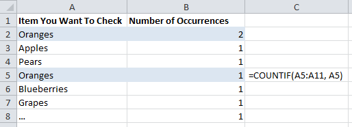
Often when working with large data sets in Excel you want to quickly identify a list of all duplicate pieces of content within a row or column. With a nice little formula and a bit of filtering this is quickly achievable. This is achieved with a simple =COUNTIF() formula as is shown below;
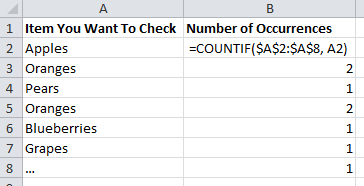
So what does all that mean? All the formula is saying is “Count the number of times the adjacent cell occurs in the whole range”. So in the example of cell B3, the formula is saying “Count the number of times the word ‘Orange’ appears within the range A2 to A8”.
Why are there dollar $ signs wrapped around the first part of the formula? This is simply telling Excel that this range is fixed. By default when you drag a formula down, all of the corresponding parts of the formula are also dragged down too, so if the dollar sign wasn’t included then then you drag down the list the results may be different as shown in another similar example below. As you can see, the results for what you would want to show the same answer are actually different – one cell says there are two occurrences of ‘Oranges’ while the other says that there is only one;
The next step that you have counted the number of occurrences of text in a range is to filter this data out by selecting the whole of Row 1 then clicking on Data > Filter as shown below;

This will then allow you to filter by showing all rows that have a number greater than 1. If you click on the small drop down arrow, then onNumber Filters, then on Greater Than then you will be able to enter in data as shown below;
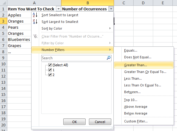
Once you click this you will be presented with an input box where you can type the number 1 into this box then press OK so that the applied filter will show just the data you require;

Now that this filter has been applied correctly you will see all the rows which have multiple occurrences within the whole column as shown below;

The next and final step is to simply copy and paste all of the filtered data from column A into a new tab on the spreadsheet. From there you can then select the whole of column A in the new tab and select Data > Remove Duplicates from the Excel menu as shown below;

This will now leave you with a final list of unique items which occur multiple times in a range of data. Quite simple really and it can have many practical uses;

This type of work can be really useful when you need to find out what specific pages on a website have duplicate content on them or other similar tasks such as duplicate title tags or meta descriptions etc. There are endless ways that this can be used so this should provide as a starting point to guide you on some of the more useful Excel functions and opportunities.
 Below is what it looks like when using the latest version with all of the pieces of data you have scraped separated by a semi-colon ;




I knew TRUE was a waste of time! I’ve tried to implement it to be useful for this purpose so many times, but it’s completely useless!!!
Thank you so much for this!
You probably could add the point that you can leave the wildcard off either side if you know that the string you’re looking for is a prefix or suffix to the data in the table_array (i.e. the start of a postal code etc.).
Great tip Max!
This solved my problem well where the middle part is text but it doesn’t work with numbers. For example in my specific case one of the partial numbers I want to look up is 50001 and the target value in the search range is 50001.801. Using *50001* returns #N/A
I have a mixture of text and numbers so I need a solution that deals with both. Any suggestions?
Thanks
Further investigation into my problem reveals that in order for the partial lookup to work it’s not the value being looked up that needs to be text it is in fact the look up range. I have used “text to columns” to convert the numbers to text and now the partial lookup works perfectly for both numbers AND text so my problem is solved in a round about way. To save the extra step it would be nice to have a formula that deals with both if you know the answer!
Hi Bob,
Yes I see the problem and solution. I’ve had a play around with doing all of this in a single formula although haven’t managed to get that working yet. This is the inherent problem when working in Excel for things like this. It’s good up until a point, whereby an SQL database would be better as it is more flexible. There is the TEXT() formula, although this still stores the data as a ‘number’ and not as a ‘string’, it simply changes the visual formatting of the text opposed to actually changing the type of content that it is stored as.
If you do find a solution to this, do pop back and let me know though
Thanks
Michael
Hi,
Thanks for this! Is there any way to tweak the formula so it searches on part of what is in cell A?
E.G. in Cell A1 I have a text string like BXXXX-1XX-XX
What I want to search for in the range is anything that matches only the BXXXX part and disregards the remainder of the value in Cell A1, and returns the value of column 3 in the range.Do you know if this is possible?
Thanks,
Babs
Hi Babs,
Yes this is possible. Rather than trying to do all of this in one mammoth formula (which is possible if you like), it may be easier to split the lookup column based on the ‘-‘, then you can simply lookup that column instead which will be the first bit you are looking for. A VLOOKUP will return the whole cell, so while the lookup on a mammoth formula would work, it would still return the whole contents of the cell where the result has been found.
Hope that helps
Great explanation, thanks! (And I also feel validated reading your opinion of TRUE in a vooklup!)
I was looking for just this very thing! I went down a number of pathways, but your answer was very simple and elegant….I studied math in college and I appreciate a simple and elegant answer. In particular, your CONCATENATE(“*”,A2,”*”) really helped me out. I needed a way to embed the actual cell reference within the wildcards. Great job and thanks!
Glad you found it useful Max
Michael,
i’m trying to work this backward. IE. I have a list with “Jim Bob (12234)” and need to lookup Jim Bob in the longer list. Limiting the # of characters from left to right will help but some first_last name combos are much longer than others. If i restrict it to 7 characters to work for “Jim bob” it will find him, but it will pull all of the instances of Rachael regardless of last name. is there a way to capture everything up to a certian character… ie “(”
thanks
You could use the MID function along with FIND which would replace the static lookup value. See here for an idea for how to use – “How To Get The Domain Name From a URL in Excel”,http://www.michaelcropper.co.uk/seo-tools/excel-tips-tricks-for-seo.
That said, the above solution isn’t that great. What I’d recommend is to split out your data using the Text to Columns button in the Excel navigation and structure your data better. I.e. 3 columns, First Name, Surname, Customer ID. Then you can look things up better.
I have a master class list that I am creating that will contain columns for Group #, Day (there will be three different training days), Date, Location, Time, and Instructor. I want to be able to list multiple groups in the group numbers column. My goal is on subsequent worksheets have the groups class information reorganized based on there number and which day of the series the class is. So the columns would look like Group #, Day 1- Date, Day 1-Location, Day 1-Time, Day 2- Date, Day 2-Location, Day 2-Time, Day 3- Date, Day 3-Location, Day 3-Time.
The reason this is so complicated and important to be able to break it down is that different groups will be combined in different days of the class. Example on day one 5/22 it might be groups 1, 2,3 but on day two for group 2 they might be joined by 5 & 6 and day three might be even different combos. I need to be able to say group 2 here are your three days in an easy way.
Thank you.
If you need to look up data which could be in multiple columns this is difficult as the VLOOKUP formula looks at the first column and brings back any column you choose once this data has been found. I’d suggest re-organising your initial lookup master list so that it just has something like; Group Number | Day | Date | Location | Time | Instructor. Then for anyone in “Group 1” (i.e. the lookup value) then you can pull all of the required information where ever you like.
I have it organized similar to what you suggest but in the Group Number box there is multiple groups. I need it to search in the array of those group values to find a specific group. Once if finds those values I want it to populate the list on a different page.
If you want ‘something’ to run through same data, then populate this data into another Sheet then you need to be using Visual Basic to run a script to do this. Formulas are used to pull data into a specific cell or range of cells. To push data into ‘somewhere’ (a Sheet or a Cell) then you need to be using VB to do this which is fun to work with.
Depending on the scale of your application, maybe it would be worth looking at a real database solution such as MySQL?
I need to use partial search, but in vice a versa way.
I have in Tab 1 general data (column A product type; column B price; column C category):
product type price category
456389 600 a
4A578964 500 b
35289 700 b
and in Tab 2 list of products
product
456389aa
4A57896478
35289ee
456389ab
35289ec
How could I get price and category behind each product in Tab 2?
Just use a normal VLOOKUP on Sheet 2, columns B and C;
B2 (Price)…….=VLOOKUP(Sheet1!A2, Sheet2!A2:B2, 2, false)
C2 (Category)….=VLOOKUP(Sheet1!A2, Sheet2!A2:B3, 3, false)
As long as there is a match for A1 in both Sheet 1 and Sheet 2, then data will match OK.
I used this formula but it causes error in excel 2003
=VLOOKUP(CONCATENATE(“*”, A2, “*”),A37:B67,2,FALSE)
What is the error you are receiving? I can’t remember ever trying this in a version as old as 2003 so I have nothing to compare with.
Hi Michael,
Please can you assist me with a formula to VLOOKUP (A1 – which is a 5 or 6 digit number) from a the 1st 5 or 6 digits of a text and bring back the comment in the same row
If I have understood correctly, this should work;
=VLOOKUP(CONCATENATE(“*”, {the cell you want to lookup on partial match}, “*”), {the rows/columns you want to find the value in – the first column is the lookup column}, {the column number you want to look up, i.e. if you are in C2 is the first column and you want to bring back D2, then this number would be set to 2}, false)
Dear Michael, thank you so much for posting this! It helped me quite a bit! However, just wanted to ask you this:
When I try to look up ALWAYS PLASTICS COMPARY in a list that contains:
ALWAYS PLASTIC COMPANY
ALWAYS PLASTIC COMPANY(I)
ALWAYS PLASTICS CO (LF)
I don’t get a match, and I found out because I am looking up COMPARY with an R and also I have PLASTICS with an S at the end. What would you recommend in this situation? The same thing happens when I look up ALL IN 1 PRODUCTS LTD in a list that contains:
ALL IN 1 LTD
Hi Dan,
Glad this has been of some use to you. Yes, you will find that if you are working with extremely bad data that any kind of VLOOKUP just isn’t going to be suitable. Really, what you need is to run through your data and clean it all up, which is unfortunately often a time consuming and manual(ish) job. Depending on what you are trying to do with this, it may be best to use an actual database (i.e. MySQL or similar) to accomplish your task. Bad data is very difficult to work with, so it would always be recommended to clean this up so that you can use the data well. Regular expression matching is possible within Excel, although it’s not straight forward,http://stackoverflow.com/questions/22542834/how-to-use-regular-expressions-regex-in-microsoft-excel-both-in-cell-and-loops.
Hope that helps anyhow, let me know if you need any other pointers.
Hi Michael, I am wondering if I am having the same question as some previous folks.
I have column a and column b.
Column A is a short list of company name I want to match up to Column B longer list of company names.
The problem is it needs to be a partial match because some of the companies will be worded slightly differently – say Institute of California and then California Institute.
Is it possible to have column c pull out from column b the likely match from column a?
Thanks!
Kat
Hi Kat,
The only way of doing this is to lookup a single word or phrase that is definitely going to be in the list. In that example you gave, “California” is always in the list. the problem being is that Column A is “Institute of California” and I’m guessing cell A2 could then be “San Francisco Institute” (the opposite of the first row).
It sounds like a bad data problem again unfortunately. When using VLOOKUP using partial match, you need to have a defined point that can be checked.
Hi Michael,
I need your help as well. I have a long list of contact numbers from different countries and I need to match them with their respective country names. I defined a group with the international codes and their country names. Now I want a formula that only looks for the first 3 or 4 integers of the phone numbers (as theses are international codes) in the contact list to match with the international codes defined by me and pull the name of the country for each.
I defined the group in both column A (International code) and B (Country name) and the list of phone numbers is in column C. I need the to see the country names in column D.
Please assist with the formula. Thank you
Hi AJ,
Ok here is what I would do. Firstly, see about splitting Column C for the phone numbers into two columns, Column C for the country code portion of the phone number, and Column D for the rest of the phone number. This may take a bit of fiddling to get this data right but it will be much easier to then look up the correct info. So once you have, Column C for the Country Code Part of Phone Number, and Column D for the Phone Number, you can then run a standard VLOOKUP in Column E for “Country Name” which is along the lines of =VLOOKUP(C2, $A$1:$A$1000, 2, false), which should pull back the relevant country name.
You could probably achieve the same thing with an enormous function trying to cram this in to take into account 3, 4, hyphenated country codes etc. but this is just a pain. So I’d recommend cleaning the data a little first to make your life easier.
Hope that helps
Perfect, just what I’ve been looking for! Thanks!
Hi Michael,
I try to use the formula that you gave but it didn’t work in my excel sheet. For example, I try lookup these names:
Jaspal Gurdev
Nurul Amira Ahmad
…… in a list that contains:
Nurul Amira binti Ahmad
Jaspal s/o Gurdev
but it give me N/A values. I try to use LEFT and Vlookup together,
but still it didn’t working out. Any suggestion?
Thanks!
Hi Dira,
You’ll have trouble trying to do that. When you don’t have the full string to lookup it is difficult. If you had in th elist “Nurul Amira Ahmad binti” and “Jaspal Gurdev s/o” then this would be simple. The only other option you have would be to split the names into different columns first, so “Jaspal” and “Gurdev” then use a “*”, “Jaspal”, “*”, “Gurdev”, “*” approach although this is going to bring back some horrible results. I’d look at cleaning your data first as there is no guarantee that there isn’t another “Jaspal Bob Gurdev” in the lookup table which would bring back the wrong results than you were expecting.
Hope that helps
Michael – outstanding information. I have implemented this for VLOOKUP for – ahem – a Fantasy Football Draft board that yields on to a team roster after the selection is made. I am dealing with one column (to simplify), and (example) I want to pull the Quarter Backs (via another formula set as “QB”). The concatenate is great for the partial and will pull the 1st RB but I have tried everything to pull the 2nd etc and cannot even after using VLOOKUP, and a combo of INDEX/MATC. SMALLIF does not work because I really need text output. As an example Matt Ryan QB is put on the draft sheet, and is pulled over on to the Roster sheet with this code:
=VLOOKUP(CONCATENATE(“*”,$B$12), Draft!G3:G17,1,FALSE)
But I cannot get a formula to pull the next QB (Tom Brady) even after experimenting with the “+1),2)” and many iterations. Any fix here?
Thanks, Andy
“pull first QB” not RB
Hi Andy,
Glad you found the information useful. So to look at your query, here’s what I’d do. The following INDEX/MATCH combo works quite well to pull the next result of something without using VLOOKUP, “=INDEX(A2:A7, MATCH(C2, A2:A7)+1)” – Whereby you are looking to MATCH the value in “C2” from the array in “A2:A7”, then moving it down one with the “+1” in the INDEX part of the formula.
The other option would be to re-jig the data a bit to add in some unique lookup values. For example, (I know nothing about English football, never mind American football!), if there are 2 Quarter Backs, could you not add in another column in the Team Roster table where you have Column A for all of the positions available in the team, then Column B would be an option to enter in the persons name, then Column C would be any other info you require to pull in about this person based on the unique lookup id of the person’s name?
Another option may be to look at how to VLOOKUP inside a VLOOKUP
Hope that helps get you on the right track