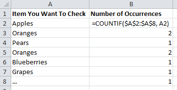
Often when working with large data sets in Excel you want to quickly identify a list of all duplicate pieces of content within a row or column. With a nice little formula and a bit of filtering this is quickly achievable. This is achieved with a simple =COUNTIF() formula as is shown below;
So what does all that mean? All the formula is saying is “Count the number of times the adjacent cell occurs in the whole range”. So in the example of cell B3, the formula is saying “Count the number of times the word ‘Orange’ appears within the range A2 to A8”.
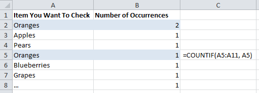
Why are there dollar $ signs wrapped around the first part of the formula? This is simply telling Excel that this range is fixed. By default when you drag a formula down, all of the corresponding parts of the formula are also dragged down too, so if the dollar sign wasn’t included then then you drag down the list the results may be different as shown in another similar example below. As you can see, the results for what you would want to show the same answer are actually different – one cell says there are two occurrences of ‘Oranges’ while the other says that there is only one;
The next step that you have counted the number of occurrences of text in a range is to filter this data out by selecting the whole of Row 1 then clicking on Data > Filter as shown below;
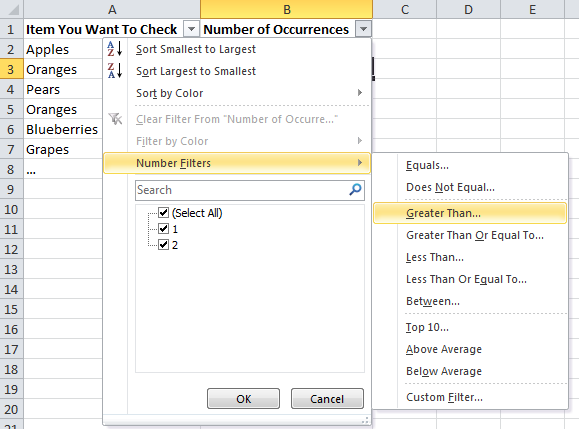
This will then allow you to filter by showing all rows that have a number greater than 1. If you click on the small drop down arrow, then onNumber Filters, then on Greater Than then you will be able to enter in data as shown below;
Once you click this you will be presented with an input box where you can type the number 1 into this box then press OK so that the applied filter will show just the data you require;
Now that this filter has been applied correctly you will see all the rows which have multiple occurrences within the whole column as shown below;
The next and final step is to simply copy and paste all of the filtered data from column A into a new tab on the spreadsheet. From there you can then select the whole of column A in the new tab and select Data > Remove Duplicates from the Excel menu as shown below;
This will now leave you with a final list of unique items which occur multiple times in a range of data. Quite simple really and it can have many practical uses;
This type of work can be really useful when you need to find out what specific pages on a website have duplicate content on them or other similar tasks such as duplicate title tags or meta descriptions etc. There are endless ways that this can be used so this should provide as a starting point to guide you on some of the more useful Excel functions and opportunities.
Michael Cropper
Latest posts by Michael Cropper (see all)
- General Scheme of the Regulation of Artificial Intelligence Bill 2026 - February 4, 2026
- WGET for Windows - April 10, 2025
- How to Setup Your Local Development Environment for Java Using Apache NetBeans and Apache Tomcat - December 1, 2023


